NEACRP C1 Rod Ejection Accident

Inputs

• rod_worth: Reactivity worth of the rod being ejected

• beta: Delayed neutron fraction

• h_gap: Gap conductancce (\(\frac{W}{m^2 \cdot K}\))

• gamma_frac: Direct heating fraction

Outputs

• max_power: Peak power reached during transient (\(\% FP\))

• burst_width: Width of power burst (\(s\))

• max_TF: Max fuel centerline temperature (\(K\))

• avg_Tcool: Average coolant temperature at outlet (\(K\))

The NEACRP C1 rod ejection accident (REA) data represents one benchmark for reactor transient analysis. The data set is used to find the relationship between the REA/reactor parameters and the power/thermal behavior of the system during/after the event. Therefore, the data set is constructed by perturbing the inputs listed above. The corresponding output results in values of interest to the safety analysis of the transient. The data were generated using deterministic simulations by the PARCS code, where the data set size includes 2000 simulations/samples [1]. The goal is to use pyMAISE to build, tune, and compare various ML models’ performance in predicting the transient outcomes based on the REA properties.

import pyMAISE as mai
import time
import pandas as pd
import numpy as np
import matplotlib.pyplot as plt
from matplotlib.gridspec import GridSpec
from scipy.stats import uniform, randint, norm
from sklearn.model_selection import ShuffleSplit
from statistics import stdev, mean

# Plot settings
matplotlib_settings = {
    "font.size": 14,
    "legend.fontsize": 12,
}
plt.rcParams.update(**matplotlib_settings)

pyMAISE Initialization

First we initialize pyMAISE with the following 4 parameters:

• verbosity: 0 \(\rightarrow\) pyMAISE prints no outputs,

• random_state: None \(\rightarrow\) No random seed is set,

• test_size: 0.3 \(\rightarrow\) 30% of the data is used for testing,

• num_configs_saved: 5 \(\rightarrow\) The top 5 hyper-parameter configurations are saved for each model.

With pyMAISE initialized we can load the preprocessor for this data set using load_rea().

global_settings = mai.settings.init()
preprocessor = mai.load_rea()

As stated the data set consists of 4 inputs:

preprocessor.inputs.head()

	rod_worth	beta	h_gap	gamma_frac
0	0.008638	0.007576	13727.981902	0.023957
1	0.009255	0.007529	9370.218080	0.019707
2	0.008046	0.007647	9962.543845	0.020045
3	0.008463	0.007139	8569.910206	0.020072
4	0.008641	0.007575	12813.925869	0.011449

and 4 outputs with 2000 total data points:

preprocessor.outputs.head()

	max_power	burst_width	max_Tf	avg_Tcool
0	181.210	0.315	918.3	561.119081
1	474.590	0.250	965.2	562.030035
2	44.083	0.425	875.7	560.194700
3	270.500	0.290	938.2	561.241696
4	195.560	0.315	924.8	561.106714

Prior to constructing any models we can get a surface understanding of the data set with a correlation matrix.

fig, ax = plt.subplots(figsize=(15,10))
fig, ax = preprocessor.correlation_matrix(fig=fig, ax=ax, annotations=True, colorbar=False)

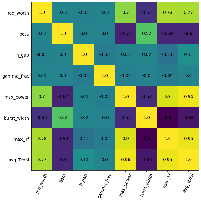
There is a positive correlation between rod worth and maximum power, maximum fuel centerline temperature, and average coolant outlet temperature. Additionally, the delayed neutron fraction correlates with burst width.

The final step of the pyMAISE initialization process is data scaling. For this data set we will use min-max scaling.

data = preprocessor.min_max_scale()

Model Initialization

We will examine the performance of 6 models in this data set:

• Linear regression: linear,

• Lasso regression: lasso,

• Decision tree regression: dtree,

• Random forest regression: rforest,

• K-nearest neighbors regression: knn,

• Sequential dense neural networks: nn.

For hyper-parameter tuning, each model must be initialized. We will use the Scikit-learn defaults for the classical ML models (linear, lasso, dtree, rforest, and knn); therefore, they are only specified in the models parameter of the model_settings dictionary. However, we must specify nn model parameters that define the layers, optimizer, and training.

model_settings = {
    "models": ["linear", "lasso", "dtree", "knn", "rforest", "nn"],
    "nn": {
        # Sequential
        "num_layers": 4,
        "dropout": True,
        "rate": 0.5,
        "validation_split": 0.15,
        "loss": "mean_absolute_error",
        "metrics": ["mean_absolute_error"],
        "batch_size": 8,
        "epochs": 75,
        "warm_start": True,
        "jit_compile": False,
        # Starting Layer
        "start_num_nodes": 100,
        "start_kernel_initializer": "normal",
        "start_activation": "relu",
        "input_dim": preprocessor.inputs.shape[1], # Number of inputs
        # Middle Layers
        "mid_num_node_strategy": "linear", # Middle layer nodes vary linearly from 'start_num_nodes' to 'end_num_nodes'
        "mid_kernel_initializer": "normal",
        "mid_activation": "relu",
        # Ending Layer
        "end_num_nodes": preprocessor.outputs.shape[1], # Number of outputs
        "end_activation": "linear",
        "end_kernel_initializer": "normal",
        # Optimizer
        "optimizer": "adam",
        "learning_rate": 5e-4,
    },
}
tuning = mai.Tuning(data=data, model_settings=model_settings)

Hyper-parameter Tuning

We will use random search for the hyper-parameter tuning of the classical models (lasso, dtree, rforest, and knn) through the random_search function. linear will be manually fit with the Scikit-learn defaults. For each classical model 300 models will be produced with randomly sampled parameter configurations. For nn, bayesian search is used to optimize the hyper-parameters in 50 iterations through the bayesian_search function. Bayesian search is appealing for nn as their training can be computationally expensive. To further reduce the computational cost of nn we specify only 10 epochs which will produce less than performant models but show the optimal parameters. For both search methods we use cross-validation to reduce bias in the models from the data set. The hyper-parameter search spaces are defined in the random_search_spaces and bayesian_search_spaces dictionaries.

random_search_spaces = {
    "lasso": {
        "alpha": uniform(loc=0.0001, scale=0.0099), # 0.0001 - 0.01
    },
    "dtree": {
        "max_depth": randint(low=5, high=50), # 5 - 50
        "max_features": [None, "sqrt", "log2", 2, 4, 6],
        "min_samples_split": randint(low=2, high=20), # 2 - 20
        "min_samples_leaf": randint(low=1, high=20), # 1 - 20
    },
    "rforest": {
        "n_estimators": randint(low=50, high=200), # 50 - 200
        "criterion": ["squared_error", "absolute_error", "poisson"],
        "min_samples_split": randint(low=2, high=20), # 2 - 20
        "min_samples_leaf": randint(low=1, high=20), # 1 - 20
        "max_features": [None, "sqrt", "log2", 2, 4, 6],
    },
    "knn": {
        "n_neighbors": randint(low=1, high=20), # 1 - 20
        "weights": ["uniform", "distance"],
        "leaf_size": randint(low=1, high=30), # 1 - 30
        "p": randint(low=1, high=10), # 1 - 10
    },
}
bayesian_search_spaces = {
    "nn": {
        "mid_num_node_strategy": ["constant", "linear"],
        "batch_size": [8, 64],
        "dropout": [True, False],
        "learning_rate": [1e-5, 0.01],
        "num_layers": [2, 6],
        "start_num_nodes": [25, 500],
    },
}

start = time.time()
random_search_configs = tuning.random_search(
    param_spaces=random_search_spaces,
    models=["linear"] + list(random_search_spaces.keys()),
    n_iter=300,
    cv=ShuffleSplit(n_splits=5, test_size=0.25, random_state=global_settings.random_state),
)
bayesian_search_configs = tuning.bayesian_search(
    param_spaces=bayesian_search_spaces,
    models=bayesian_search_spaces.keys(),
    n_iter=50,
    cv=ShuffleSplit(n_splits=5, test_size=0.25, random_state=global_settings.random_state),
)
stop = time.time()
print("Hyper-parameter tuning took " + str((stop - start) / 60) + " minutes to process.")

Hyper-parameter tuning search space was not provided for linear, doing manual fit
Hyper-parameter tuning took 108.24320970773697 minutes to process.

We can understand the hyper-parameter tuning of Bayesian search from the convergence plot.

fig, ax = plt.subplots(figsize=(8,8))
ax = tuning.convergence_plot(model_types="nn")

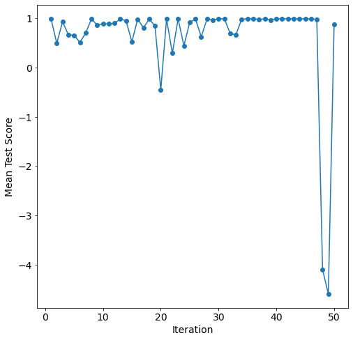
Fewer than 30 iterations were required to converge to the optimal parameter configurations.

Model Post-processing

Now that the top num_configs_saved saved, we can pass these models to the PostProcessor for model comparison and analysis. To improve the nn performance we can pass an updated epochs parameter. Using 500 epochs should improve fitting at higher computational cost.

new_model_settings = {
    "nn": {"epochs": 500}
}
postprocessor = mai.PostProcessor(
    data=data,
    models_list=[random_search_configs, bayesian_search_configs],
    new_model_settings=new_model_settings,
    yscaler=preprocessor.yscaler,
)

To compare the performance of these models we will compute 4 metrics for both the training and testing data:

• mean squared error MSE \(=\frac{1}{n}\sum^n_{i = 1}(y_i - \hat{y_i})^2\),

• root mean squared error RMSE \(=\sqrt{\frac{1}{n}\sum^n_{i = 1}(y_i - \hat{y_i})^2}\),

• mean absolute error MAE = \(=\frac{1}{n}\sum^n_{i = 1}|y_i - \hat{y_i}|\),

• and r-squared R2 \(=1 - \frac{\sum^n_{i = 1}(y_i - \hat{y_i})^2}{\sum^n_{i = 1}(y_i - \bar{y_i})^2}\),

where \(y\) is the actual outcome, \(\bar{y}\) is the average outcome, \(\hat{y}\) is the model predicted outcome, and \(n\) is the number of observations. The averaged performance metrics are shown below.

postprocessor.metrics()[["Model Types", "Train R2", "Test R2"]]

	Model Types	Train R2	Test R2
22	nn	0.996991	0.996563
25	nn	0.997542	0.996274
23	nn	0.993635	0.994332
21	nn	0.994222	0.993968
24	nn	0.990929	0.991919
12	rforest	0.995286	0.986470
11	rforest	0.996907	0.986128
13	rforest	0.993114	0.984042
15	rforest	0.990654	0.983169
14	rforest	0.990818	0.981383
7	dtree	0.998771	0.960748
6	dtree	1.000000	0.960440
10	dtree	0.995147	0.959554
9	dtree	0.997734	0.956914
8	dtree	0.999312	0.955705
19	knn	1.000000	0.949050
17	knn	1.000000	0.948966
16	knn	1.000000	0.947115
18	knn	1.000000	0.946237
20	knn	0.950356	0.939592
0	linear	0.854579	0.850833
4	lasso	0.854311	0.850303
1	lasso	0.854212	0.850150
2	lasso	0.854065	0.849899
3	lasso	0.854057	0.849886
5	lasso	0.853920	0.849656

Given the top performing models are linear and lasso this data set’s outputs are linear with their inputs. nn also performs well with all models greater than 0.95. Performance quickly drops off with rforest, knn, and dtree. We can look specifically at the performance for each output:

postprocessor.metrics(y="max_power")

	Model Types	Parameter Configurations	Train R2	Train MAE	Train MSE	Train RMSE	Test R2	Test MAE	Test MSE	Test RMSE
21	nn	{'batch_size': 8, 'dropout': 0, 'learning_rate...	0.999765	2.133878	10.063103	3.172239	0.999828	2.030514	7.801756	2.793162
22	nn	{'batch_size': 8, 'dropout': 0, 'learning_rate...	0.999833	2.112485	7.136338	2.671393	0.999809	2.219746	8.629569	2.937613
23	nn	{'batch_size': 13, 'dropout': 0, 'learning_rat...	0.999527	3.283176	20.276449	4.502938	0.999619	3.345278	17.225367	4.150345
25	nn	{'batch_size': 21, 'dropout': 0, 'learning_rat...	0.999574	3.959537	18.271895	4.274564	0.999582	3.942873	18.888371	4.346075
24	nn	{'batch_size': 8, 'dropout': 0, 'learning_rate...	0.999397	3.839394	25.836482	5.082960	0.999391	3.985900	27.552767	5.249073
12	rforest	{'criterion': 'poisson', 'max_features': None,...	0.998844	3.694867	49.532222	7.037913	0.991611	10.021148	379.428960	19.478936
11	rforest	{'criterion': 'squared_error', 'max_features':...	0.998732	4.066483	54.318439	7.370104	0.990279	10.491619	439.651007	20.967857
14	rforest	{'criterion': 'absolute_error', 'max_features'...	0.996685	6.143280	142.022579	11.917323	0.989230	11.197654	487.118868	22.070770
15	rforest	{'criterion': 'squared_error', 'max_features':...	0.997262	5.726082	117.322278	10.831541	0.988743	11.284735	509.128735	22.563881
13	rforest	{'criterion': 'poisson', 'max_features': 6, 'm...	0.997948	4.804165	87.931383	9.377174	0.987344	11.140833	572.401047	23.924904
10	dtree	{'max_depth': 23, 'max_features': None, 'min_s...	0.997487	6.092556	107.659430	10.375906	0.979565	19.109739	924.216361	30.400927
7	dtree	{'max_depth': 30, 'max_features': 6, 'min_samp...	0.999503	2.354660	21.306076	4.615851	0.978051	20.263113	992.725335	31.507544
6	dtree	{'max_depth': 31, 'max_features': None, 'min_s...	1.000000	0.000000	0.000000	0.000000	0.977857	20.057878	1001.494090	31.646391
9	dtree	{'max_depth': 37, 'max_features': 6, 'min_samp...	0.998593	4.222973	60.297608	7.765153	0.975976	20.147429	1086.564282	32.963075
8	dtree	{'max_depth': 11, 'max_features': 6, 'min_samp...	0.999548	2.004389	19.346764	4.398496	0.973210	21.389837	1211.670836	34.809063
17	knn	{'leaf_size': 28, 'n_neighbors': 5, 'p': 2, 'w...	1.000000	0.000000	0.000000	0.000000	0.971296	21.422576	1298.217237	36.030782
19	knn	{'leaf_size': 9, 'n_neighbors': 3, 'p': 2, 'we...	1.000000	0.000000	0.000000	0.000000	0.970830	22.624646	1319.297694	36.322138
16	knn	{'leaf_size': 7, 'n_neighbors': 4, 'p': 2, 'we...	1.000000	0.000000	0.000000	0.000000	0.970633	22.012378	1328.196327	36.444428
18	knn	{'leaf_size': 18, 'n_neighbors': 6, 'p': 2, 'w...	1.000000	0.000000	0.000000	0.000000	0.970355	21.527457	1340.782022	36.616690
20	knn	{'leaf_size': 1, 'n_neighbors': 5, 'p': 4, 'we...	0.973073	18.921449	1153.640964	33.965291	0.964079	23.701504	1624.645752	40.306895
0	linear	{'copy_X': True, 'fit_intercept': True, 'n_job...	0.883119	50.664327	5007.516923	70.763811	0.877886	52.341080	5522.919504	74.316347
4	lasso	{'alpha': 0.00015499889632899263}	0.882972	50.615358	5013.822766	70.808352	0.877659	52.333832	5533.217815	74.385602
1	lasso	{'alpha': 0.00018375666615060612}	0.882912	50.612206	5016.379778	70.826406	0.877585	52.341321	5536.563923	74.408090
2	lasso	{'alpha': 0.00022582145708762807}	0.882806	50.612246	5020.901953	70.858323	0.877459	52.357448	5542.267588	74.446407
3	lasso	{'alpha': 0.00022794412681753656}	0.882800	50.612303	5021.154770	70.860107	0.877452	52.358437	5542.580883	74.448512
5	lasso	{'alpha': 0.0002627188109898158}	0.882696	50.615824	5025.633335	70.891701	0.877331	52.374636	5548.061975	74.485314

For max power all but linear and lasso did well.

postprocessor.metrics(y="burst_width")

	Model Types	Parameter Configurations	Train R2	Train MAE	Train MSE	Train RMSE	Test R2	Test MAE	Test MSE	Test RMSE
22	nn	{'batch_size': 8, 'dropout': 0, 'learning_rate...	0.988799	0.005160	0.000172	0.013098	0.987108	0.005698	0.000239	0.015456
25	nn	{'batch_size': 21, 'dropout': 0, 'learning_rat...	0.991330	0.005005	0.000133	0.011524	0.986333	0.005875	0.000253	0.015914
23	nn	{'batch_size': 13, 'dropout': 0, 'learning_rat...	0.977841	0.005919	0.000339	0.018422	0.980524	0.006991	0.000361	0.018997
21	nn	{'batch_size': 8, 'dropout': 0, 'learning_rate...	0.978727	0.006273	0.000326	0.018050	0.977655	0.007223	0.000414	0.020349
12	rforest	{'criterion': 'poisson', 'max_features': None,...	0.985973	0.002829	0.000215	0.014657	0.974381	0.006673	0.000475	0.021788
11	rforest	{'criterion': 'squared_error', 'max_features':...	0.992650	0.003202	0.000113	0.010610	0.973837	0.006776	0.000485	0.022018
13	rforest	{'criterion': 'poisson', 'max_features': 6, 'm...	0.982523	0.004071	0.000268	0.016361	0.973693	0.006995	0.000487	0.022079
24	nn	{'batch_size': 8, 'dropout': 0, 'learning_rate...	0.967319	0.007959	0.000501	0.022373	0.971284	0.008661	0.000532	0.023067
15	rforest	{'criterion': 'squared_error', 'max_features':...	0.975306	0.004684	0.000378	0.019448	0.968105	0.007372	0.000591	0.024311
14	rforest	{'criterion': 'absolute_error', 'max_features'...	0.978055	0.004783	0.000336	0.018333	0.961587	0.007456	0.000712	0.026679
6	dtree	{'max_depth': 31, 'max_features': None, 'min_s...	1.000000	0.000000	0.000000	0.000000	0.915653	0.013175	0.001563	0.039534
7	dtree	{'max_depth': 30, 'max_features': 6, 'min_samp...	0.997753	0.001886	0.000034	0.005866	0.915387	0.013296	0.001568	0.039597
10	dtree	{'max_depth': 23, 'max_features': None, 'min_s...	0.990948	0.004050	0.000139	0.011774	0.908150	0.013236	0.001702	0.041255
8	dtree	{'max_depth': 11, 'max_features': 6, 'min_samp...	0.999439	0.001429	0.000009	0.002932	0.906660	0.013048	0.001730	0.041589
9	dtree	{'max_depth': 37, 'max_features': 6, 'min_samp...	0.997002	0.002823	0.000046	0.006776	0.902873	0.013235	0.001800	0.042424
19	knn	{'leaf_size': 9, 'n_neighbors': 3, 'p': 2, 'we...	1.000000	0.000000	0.000000	0.000000	0.873178	0.015211	0.002350	0.048477
17	knn	{'leaf_size': 28, 'n_neighbors': 5, 'p': 2, 'w...	1.000000	0.000000	0.000000	0.000000	0.868704	0.014066	0.002433	0.049325
16	knn	{'leaf_size': 7, 'n_neighbors': 4, 'p': 2, 'we...	1.000000	0.000000	0.000000	0.000000	0.863291	0.014743	0.002533	0.050331
18	knn	{'leaf_size': 18, 'n_neighbors': 6, 'p': 2, 'w...	1.000000	0.000000	0.000000	0.000000	0.860476	0.014414	0.002585	0.050847
20	knn	{'leaf_size': 1, 'n_neighbors': 5, 'p': 4, 'we...	0.867813	0.012254	0.002025	0.044995	0.847149	0.015478	0.002832	0.053220
0	linear	{'copy_X': True, 'fit_intercept': True, 'n_job...	0.568566	0.035066	0.006608	0.081288	0.561224	0.038123	0.008131	0.090170
4	lasso	{'alpha': 0.00015499889632899263}	0.567971	0.033968	0.006617	0.081344	0.559685	0.037069	0.008159	0.090328
1	lasso	{'alpha': 0.00018375666615060612}	0.567766	0.033770	0.006620	0.081363	0.559282	0.036893	0.008167	0.090369
2	lasso	{'alpha': 0.00022582145708762807}	0.567522	0.033493	0.006624	0.081386	0.558636	0.036641	0.008179	0.090435
3	lasso	{'alpha': 0.00022794412681753656}	0.567510	0.033479	0.006624	0.081387	0.558603	0.036628	0.008179	0.090439
5	lasso	{'alpha': 0.0002627188109898158}	0.567299	0.033254	0.006627	0.081407	0.558036	0.036421	0.008190	0.090497

For burst width knn, dtree, lasso, and linear struggled to predict the testing data. knn overfit to the training data set.

postprocessor.metrics(y="max_Tf")

	Model Types	Parameter Configurations	Train R2	Train MAE	Train MSE	Train RMSE	Test R2	Test MAE	Test MSE	Test RMSE
22	nn	{'batch_size': 8, 'dropout': 0, 'learning_rate...	0.999606	0.476851	0.494479	0.703192	0.999593	0.514516	0.534188	0.730882
25	nn	{'batch_size': 21, 'dropout': 0, 'learning_rat...	0.999654	0.531952	0.435127	0.659641	0.999570	0.561521	0.563811	0.750873
21	nn	{'batch_size': 8, 'dropout': 0, 'learning_rate...	0.998736	0.796847	1.587985	1.260153	0.998745	0.810594	1.645989	1.282961
24	nn	{'batch_size': 8, 'dropout': 0, 'learning_rate...	0.997993	1.064926	2.520588	1.587636	0.998061	1.124524	2.543935	1.594972
23	nn	{'batch_size': 13, 'dropout': 0, 'learning_rat...	0.997786	1.214482	2.780910	1.667606	0.997780	1.280105	2.911773	1.706392
11	rforest	{'criterion': 'squared_error', 'max_features':...	0.997825	1.095227	2.731355	1.652681	0.989698	2.461387	13.514313	3.676182
12	rforest	{'criterion': 'poisson', 'max_features': None,...	0.997872	0.985909	2.672958	1.634918	0.989633	2.511683	13.599902	3.687805
15	rforest	{'criterion': 'squared_error', 'max_features':...	0.993997	1.777071	7.538544	2.745641	0.987258	2.768031	16.714941	4.088391
13	rforest	{'criterion': 'poisson', 'max_features': 6, 'm...	0.995041	1.633966	6.227993	2.495595	0.986598	2.791944	17.581126	4.192985
14	rforest	{'criterion': 'absolute_error', 'max_features'...	0.993344	1.943850	8.359785	2.891329	0.986437	2.910056	17.792976	4.218172
0	linear	{'copy_X': True, 'fit_intercept': True, 'n_job...	0.984094	2.737370	19.975873	4.469438	0.983467	2.860855	21.688595	4.657102
4	lasso	{'alpha': 0.00015499889632899263}	0.983848	2.651807	20.285131	4.503902	0.983224	2.793339	22.007038	4.691166
1	lasso	{'alpha': 0.00018375666615060612}	0.983748	2.643162	20.410535	4.517802	0.983129	2.785325	22.131543	4.704417
2	lasso	{'alpha': 0.00022582145708762807}	0.983572	2.633487	20.632317	4.542281	0.982962	2.779027	22.350542	4.727636
3	lasso	{'alpha': 0.00022794412681753656}	0.983562	2.633147	20.644716	4.543646	0.982953	2.778929	22.362755	4.728927
5	lasso	{'alpha': 0.0002627188109898158}	0.983387	2.628571	20.864359	4.567752	0.982789	2.779341	22.578708	4.751706
17	knn	{'leaf_size': 28, 'n_neighbors': 5, 'p': 2, 'w...	1.000000	0.000000	0.000000	0.000000	0.975539	3.576428	32.088355	5.664658
16	knn	{'leaf_size': 7, 'n_neighbors': 4, 'p': 2, 'we...	1.000000	0.000000	0.000000	0.000000	0.974794	3.743922	33.066542	5.750352
18	knn	{'leaf_size': 18, 'n_neighbors': 6, 'p': 2, 'w...	1.000000	0.000000	0.000000	0.000000	0.974527	3.621026	33.416091	5.780665
10	dtree	{'max_depth': 23, 'max_features': None, 'min_s...	0.995139	1.741500	6.104337	2.470696	0.973796	4.253417	34.375232	5.863039
19	knn	{'leaf_size': 9, 'n_neighbors': 3, 'p': 2, 'we...	1.000000	0.000000	0.000000	0.000000	0.973567	3.868463	34.675625	5.888601
7	dtree	{'max_depth': 30, 'max_features': 6, 'min_samp...	0.998618	0.728214	1.735818	1.317504	0.972962	4.455750	35.469846	5.955657
6	dtree	{'max_depth': 31, 'max_features': None, 'min_s...	1.000000	0.000000	0.000000	0.000000	0.971959	4.527000	36.785733	6.065124
9	dtree	{'max_depth': 37, 'max_features': 6, 'min_samp...	0.997024	1.266952	3.737929	1.933372	0.971806	4.427972	36.986470	6.081650
20	knn	{'leaf_size': 1, 'n_neighbors': 5, 'p': 4, 'we...	0.976595	3.308671	29.394203	5.421642	0.971088	3.946267	37.927531	6.158533
8	dtree	{'max_depth': 11, 'max_features': 6, 'min_samp...	0.998946	0.623212	1.323978	1.150642	0.967522	4.624231	42.605800	6.527312

For max fuel temperature, all models were able to model this output. This indicates the max fuel temperature in linear with the inputs.

postprocessor.metrics(y="avg_Tcool")

	Model Types	Parameter Configurations	Train R2	Train MAE	Train MSE	Train RMSE	Test R2	Test MAE	Test MSE	Test RMSE
22	nn	{'batch_size': 8, 'dropout': 0, 'learning_rate...	0.999727	0.010189	0.000152	0.012345	0.999743	0.010191	0.000151	0.012292
21	nn	{'batch_size': 8, 'dropout': 0, 'learning_rate...	0.999660	0.010413	0.000190	0.013768	0.999643	0.010754	0.000210	0.014492
25	nn	{'batch_size': 21, 'dropout': 0, 'learning_rat...	0.999613	0.013282	0.000216	0.014697	0.999611	0.013677	0.000229	0.015138
23	nn	{'batch_size': 13, 'dropout': 0, 'learning_rat...	0.999386	0.014937	0.000343	0.018511	0.999404	0.015323	0.000351	0.018739
24	nn	{'batch_size': 8, 'dropout': 0, 'learning_rate...	0.999008	0.017018	0.000554	0.023529	0.998942	0.017794	0.000623	0.024961
11	rforest	{'criterion': 'squared_error', 'max_features':...	0.998422	0.019401	0.000881	0.029684	0.990699	0.046547	0.005477	0.074007
12	rforest	{'criterion': 'poisson', 'max_features': None,...	0.998453	0.018792	0.000863	0.029384	0.990254	0.049577	0.005739	0.075758
15	rforest	{'criterion': 'squared_error', 'max_features':...	0.996052	0.029694	0.002204	0.046951	0.988569	0.051719	0.006732	0.082046
13	rforest	{'criterion': 'poisson', 'max_features': 6, 'm...	0.996944	0.026526	0.001706	0.041308	0.988534	0.051929	0.006752	0.082171
14	rforest	{'criterion': 'absolute_error', 'max_features'...	0.995187	0.034239	0.002687	0.051836	0.988280	0.055895	0.006901	0.083074
0	linear	{'copy_X': True, 'fit_intercept': True, 'n_job...	0.982538	0.069947	0.009749	0.098737	0.980755	0.074340	0.011333	0.106454
4	lasso	{'alpha': 0.00015499889632899263}	0.982454	0.070464	0.009796	0.098974	0.980644	0.075362	0.011398	0.106763
1	lasso	{'alpha': 0.00018375666615060612}	0.982420	0.070589	0.009815	0.099070	0.980605	0.075581	0.011421	0.106869
2	lasso	{'alpha': 0.00022582145708762807}	0.982360	0.070788	0.009848	0.099239	0.980538	0.075904	0.011460	0.107053
3	lasso	{'alpha': 0.00022794412681753656}	0.982357	0.070799	0.009850	0.099248	0.980535	0.075920	0.011462	0.107063
5	lasso	{'alpha': 0.0002627188109898158}	0.982298	0.070972	0.009883	0.099415	0.980470	0.076199	0.011501	0.107241
17	knn	{'leaf_size': 28, 'n_neighbors': 5, 'p': 2, 'w...	1.000000	0.000000	0.000000	0.000000	0.980326	0.074259	0.011585	0.107634
16	knn	{'leaf_size': 7, 'n_neighbors': 4, 'p': 2, 'we...	1.000000	0.000000	0.000000	0.000000	0.979742	0.076561	0.011929	0.109221
18	knn	{'leaf_size': 18, 'n_neighbors': 6, 'p': 2, 'w...	1.000000	0.000000	0.000000	0.000000	0.979589	0.075897	0.012019	0.109632
19	knn	{'leaf_size': 9, 'n_neighbors': 3, 'p': 2, 'we...	1.000000	0.000000	0.000000	0.000000	0.978625	0.081296	0.012587	0.112191
9	dtree	{'max_depth': 37, 'max_features': 6, 'min_samp...	0.998319	0.019348	0.000938	0.030634	0.977002	0.085462	0.013543	0.116373
10	dtree	{'max_depth': 23, 'max_features': None, 'min_s...	0.997014	0.028430	0.001667	0.040833	0.976706	0.086039	0.013717	0.117119
7	dtree	{'max_depth': 30, 'max_features': 6, 'min_samp...	0.999210	0.011467	0.000441	0.021007	0.976592	0.085899	0.013784	0.117405
6	dtree	{'max_depth': 31, 'max_features': None, 'min_s...	1.000000	0.000000	0.000000	0.000000	0.976290	0.085863	0.013962	0.118160
20	knn	{'leaf_size': 1, 'n_neighbors': 5, 'p': 4, 'we...	0.983943	0.066562	0.008965	0.094683	0.976052	0.082846	0.014102	0.118753
8	dtree	{'max_depth': 11, 'max_features': 6, 'min_samp...	0.999315	0.010149	0.000382	0.019553	0.975428	0.087764	0.014469	0.120289

Average coolant temperature was also well predicted by all models.

We can see the parameters of each model with the best Test R2 with get_params.

for model in model_settings["models"]:
    print(postprocessor.get_params(model_type=model), "\n")

  Model Types  copy_X  fit_intercept n_jobs   normalize  positive
0      linear    True           True   None  deprecated     False

  Model Types     alpha
0       lasso  0.000155

  Model Types  max_depth  max_features  min_samples_leaf  min_samples_split
0       dtree         37             6                 1                  4

  Model Types  leaf_size  n_neighbors  p   weights
0         knn         28            5  2  distance

  Model Types      criterion  max_features  min_samples_leaf  \
0     rforest  squared_error             4                 1

   min_samples_split  n_estimators
0                  3           186

  Model Types  batch_size  dropout  learning_rate mid_num_node_strategy  \
0          nn           8        0       0.002693              constant

   num_layers  start_num_nodes
0           2              310

We can visualize the performance of each model with diagonal validation plots. These plots show the predicted output to the actual output. For the plots below we will do max burst width.

models = np.array([["linear", "lasso"], ["dtree", "knn"], ["rforest", "nn"]])

output = ["burst_width"]

fig = plt.figure(constrained_layout=fig, figsize=(10,15))
gs = GridSpec(models.shape[0], models.shape[1], figure=fig)
for i in range(models.shape[0]):
    for j in range(models.shape[1]):
        if models[i, j] != None:
            ax = fig.add_subplot(gs[i, j])
            ax = postprocessor.diagonal_validation_plot(
                model_type=models[i, j],
                y=output,
            )
            ax.set_title(models[i, j])

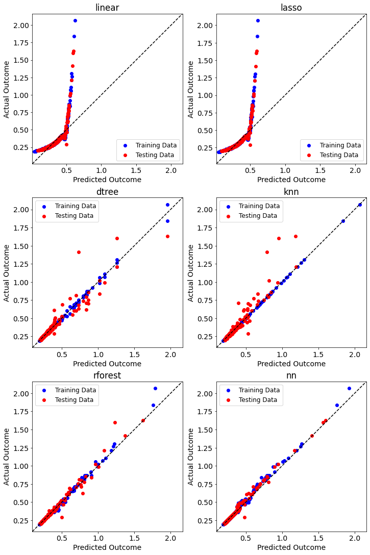
We see that all models except linear and lasso do relatively well predicting burst width. nn has the best performance according to these diagonal validation plots.

Similarly, the validation_plot function produces validation plots that show the absolute relative error for each burst width prediction.

fig = plt.figure(constrained_layout=fig, figsize=(15,20))
gs = GridSpec(models.shape[0], models.shape[1], figure=fig)
for i in range(models.shape[0]):
    for j in range(models.shape[1]):
        if models[i, j] != None:
            ax = fig.add_subplot(gs[i, j])
            ax = postprocessor.validation_plot(
                model_type=models[i, j],
                y=output,
            )
            ax.set_title(models[i, j])

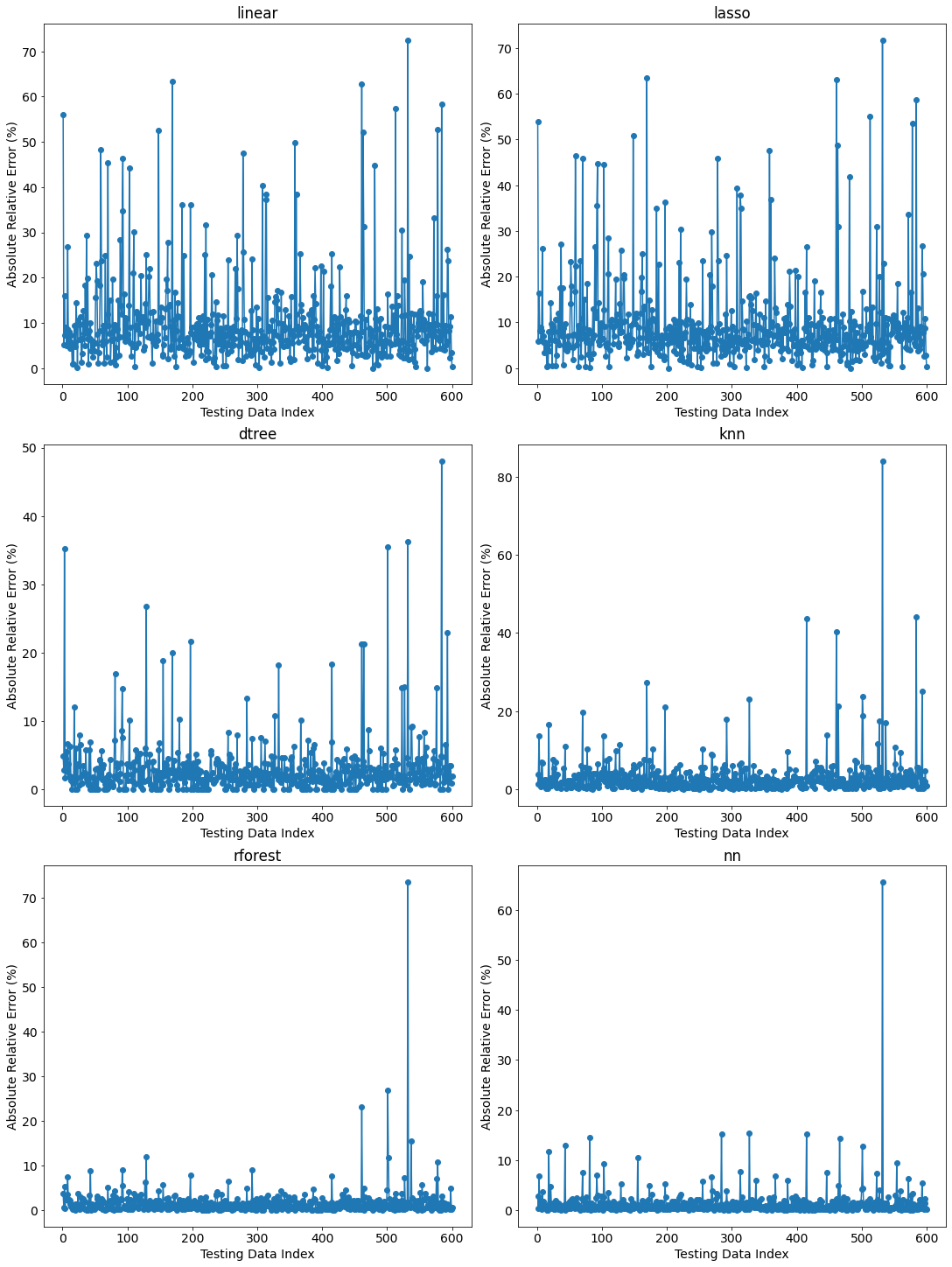
The performance gap of the linear model to the others is evident in the magnitude of the relative error.

Finally, the learning curve of the most performant nn is shown by nn_learning_plot.

fig, ax = plt.subplots(figsize=(8,8))
ax = postprocessor.nn_learning_plot()

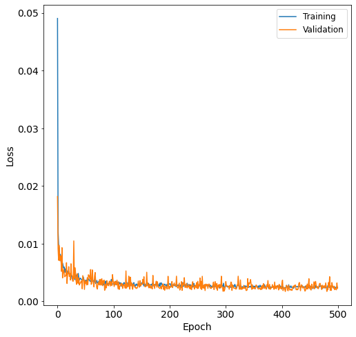
The validation curve is below the training curve; therefore, the nn is not overfit.

References

1. 8. Finnemann and A. Galati, “NEACRP 3-D LWR Core Transient Benchmark,” NEACRP-L-335, Revision 1, 1992.