Fuel Performance

Inputs

• fuel_dens: Fuel density (\(\frac{kg}{m^3}\))

• porosity: Porosity

• clad_thick: Cladding thickness (\(m\))

• pellet_OD: Pellet outer diameter (\(m\))

• pellet_h: Pellet height (\(m\))

• gap_thick: Gap thickness (\(m\))

• inlet_T: Inlet temperature (\(K\))

• enrich: U-235 enrichment

• rough_fuel: Fuel roughness (\(m\))

• rough_clad: Clad rouchness (\(m\))

• ax_pow: Axial power

• clad_T: Cladding surface temperature (\(K\))

• pressure: Pressure (\(Pa\))

Outputs

• fis_gas_produced: Fission gas production (\(mol\))

• max_fuel_centerline_temp: Max fuel centerline temperature (\(K\))

• max_fuel_surface_temp: Max fuel surface temperature (\(K\))

• radial_clad_dia: Radial cladding diameter displacement after irradiation (\(m\))

This data set consists of 13 inputs and 4 outputs with 400 data points. This data originates from [1], and a graphical representation is provided in the figure below. Case 1 from the pellet-cladding mechanical interaction (PCMI) benchmark [2] was selected for the data set. This benchmark simulates a beginning of life (BOL) ramp of a 10-pellet pressurized water reactor (PWR) fuel rod to an average linear heat rate of \(40~kW/m\). The inner and outer cladding diameters are reduced, so the fuel-clad interaction occurs during the ramp time. Axial power and rod surface temperature profiles were assumed to be uniform at \(330^\circ C\). The 13 input parameters were uniformly randomly sampled independently within their uncertainty bounds and simulated in BISON. The rod response was recorded in 4 outputs.

import pyMAISE as mai
import time
import pandas as pd
import numpy as np
import matplotlib.pyplot as plt
from matplotlib.gridspec import GridSpec
from scipy.stats import uniform, randint
from sklearn.model_selection import ShuffleSplit

# Plot settings
matplotlib_settings = {
    "font.size": 14,
    "legend.fontsize": 12,
}
plt.rcParams.update(**matplotlib_settings)

pyMAISE Initialization

First we initialize pyMAISE with the following 4 parameters:

• verbosity: 0 \(\rightarrow\) pyMAISE prints no outputs,

• random_state: None \(\rightarrow\) No random seed is set,

• test_size: 0.3 \(\rightarrow\) 30% of the data is used for testing,

• num_configs_saved: 5 \(\rightarrow\) The top 5 hyper-parameter configurations are saved for each model.

With pyMAISE initialized we can load the preprocessor for this data set using load_fp().

global_settings = mai.settings.init()
preprocessor = mai.load_fp()

As stated the data set consists of 13 inputs:

preprocessor.inputs.head()

	fuel_dens	porosity	clad_thick	pellet_OD	pellet_h	gap_thick	inlet_T	enrich	rough_fuel	rough_clad	ax_pow	clad_T	pressure
0	10466	0.040527	0.000571	0.004104	0.013077	0.000019	292.36	0.044852	0.000002	3.890000e-07	0.99967	602.72	15504000
1	10488	0.041780	0.000570	0.004096	0.014227	0.000019	291.33	0.044942	0.000002	4.170000e-07	0.98741	602.81	15591000
2	10434	0.058323	0.000568	0.004094	0.013923	0.000019	293.35	0.044889	0.000002	3.670000e-07	0.99225	620.33	15510000
3	10449	0.038379	0.000572	0.004093	0.013976	0.000019	293.29	0.044937	0.000002	3.250000e-07	1.02650	610.91	15382000
4	10429	0.038438	0.000568	0.004096	0.013787	0.000019	291.81	0.044849	0.000002	4.360000e-07	0.99289	597.05	15583000

and 4 outputs with 400 total data points:

preprocessor.outputs.head()

	fis_gas_produced	max_fuel_centerline_temp	max_fuel_surface_temp	radial_clad_dia
0	0.000029	1569.699310	699.613033	0.000019
1	0.000032	1559.465162	699.976191	0.000019
2	0.000031	1632.394103	712.771506	0.000020
3	0.000032	1613.399315	710.114032	0.000020
4	0.000031	1542.540705	694.956854	0.000018

Prior to constructing any models we can get a surface understanding of the data set with a correlation matrix.

fig, ax = plt.subplots(figsize=(15,10))
fig, ax = preprocessor.correlation_matrix(fig=fig, ax=ax)

There is a positive correlation between axial power and cladding temperature with max fuel centerline temperature, max fuel surface temperature, and radial cladding diameter. Additionally, the fission gas production correlates with pellet height.

The final step of the pyMAISE initialization process is data scaling. For this data set we will use min-max scaling.

data = preprocessor.min_max_scale()

Model Initialization

We will examine the performance of 6 models in this data set:

• Linear regression: linear,

• Lasso regression: lasso,

• Decision tree regression: dtree,

• Random forest regression: rforest,

• K-nearest neighbors regression: knn,

• Sequential dense neural networks: nn.

For hyper-parameter tuning each model must be initialized. We will use the Scikit-learn defaults for the classical ML models (linear, lasso, dtree, rforest, and knn); therefore, they are only specified in the models parameter of the model_settings dictionary. However, we must specify nn model parameters that define the layers, optimizer, and training.

model_settings = {
    "models": ["linear", "lasso", "dtree", "knn", "rforest", "nn"],
    "nn": {
        # Sequential
        "num_layers": 4,
        "dropout": True,
        "rate": 0.5,
        "validation_split": 0.15,
        "loss": "mean_absolute_error",
        "metrics": ["mean_absolute_error"],
        "batch_size": 8,
        "epochs": 50,
        "warm_start": True,
        "jit_compile": False,
        # Starting Layer
        "start_num_nodes": 100,
        "start_kernel_initializer": "normal",
        "start_activation": "relu",
        "input_dim": preprocessor.inputs.shape[1], # Number of inputs
        # Middle Layers
        "mid_num_node_strategy": "linear", # Middle layer nodes vary linearly from 'start_num_nodes' to 'end_num_nodes'
        "mid_kernel_initializer": "normal",
        "mid_activation": "relu",
        # Ending Layer
        "end_num_nodes": preprocessor.outputs.shape[1], # Number of outputs
        "end_activation": "linear",
        "end_kernel_initializer": "normal",
        # Optimizer
        "optimizer": "adam",
        "learning_rate": 5e-4,
    },
}
tuning = mai.Tuning(data=data, model_settings=model_settings)

Hyper-parameter Tuning

We will use random search for the hyper-parameter tuning of the classical models (lasso, dtree, rforest, and knn) through the random_search function. linear will be manually fit with the Scikit-learn defaults. For each classical model 300 models will be produced with randomly sampled parameter configurations. For nn, bayesian search is used to optimize the hyper-parameters in 50 iterations through the bayesian_search function. Bayesian search is appealing for nn as their training can be computationally expensive. To further reduce the computational cost of nn we specify only 10 epochs which will produce less than performant models but show the optimal parameters. For both search methods we use cross-validation to reduce bias in the models from the data set. The hyper-parameter search spaces are defined in the random_search_spaces and bayesian_search_spaces dictionaries.

random_search_spaces = {
    "lasso": {
        "alpha": uniform(loc=0.0001, scale=0.0099), # 0.0001 - 0.01
    },
    "dtree": {
        "max_depth": randint(low=5, high=50), # 5 - 50
        "max_features": [None, "sqrt", "log2", 2, 4, 6],
        "min_samples_split": randint(low=2, high=20), # 2 - 20
        "min_samples_leaf": randint(low=1, high=20), # 1 - 20
    },
    "rforest": {
        "n_estimators": randint(low=50, high=200), # 50 - 200
        "criterion": ["squared_error", "absolute_error", "poisson"],
        "min_samples_split": randint(low=2, high=20), # 2 - 20
        "min_samples_leaf": randint(low=1, high=20), # 1 - 20
        "max_features": [None, "sqrt", "log2", 2, 4, 6],
    },
    "knn": {
        "n_neighbors": randint(low=1, high=20), # 1 - 20
        "weights": ["uniform", "distance"],
        "leaf_size": randint(low=1, high=30), # 1 - 30
        "p": randint(low=1, high=10), # 1 - 10
    },
}
bayesian_search_spaces = {
    "nn": {
        "mid_num_node_strategy": ["constant", "linear"],
        "batch_size": [8, 64],
        "learning_rate": [1e-5, 0.001],
        "num_layers": [2, 6],
        "start_num_nodes": [25, 300],
    },
}

start = time.time()
random_search_configs = tuning.random_search(
    param_spaces=random_search_spaces,
    models=["linear"] + list(random_search_spaces.keys()),
    n_iter=300,
    cv=ShuffleSplit(n_splits=5, test_size=0.25, random_state=global_settings.random_state),
)
bayesian_search_configs = tuning.bayesian_search(
    param_spaces=bayesian_search_spaces,
    models=bayesian_search_spaces.keys(),
    n_iter=50,
    cv=5,
)
stop = time.time()
print("Hyper-parameter tuning took " + str((stop - start) / 60) + " minutes to process.")

Hyper-parameter tuning search space was not provided for linear, doing manual fit
Hyper-parameter tuning took 25.628323105971017 minutes to process.

We can understand the hyper-parameter tuning of Bayesian search from the convergence plot.

fig, ax = plt.subplots(figsize=(8,8))
ax = tuning.convergence_plot(model_types="nn")

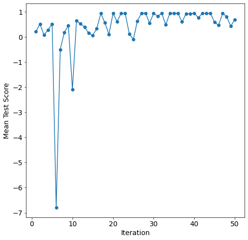
Fewer than 30 iterations were required to converge to the optimal parameter configurations.

Model Post-processing

Now that the top num_configs_saved saved, we can pass these models to the PostProcessor for model comparison and analysis. To improve the nn performance we can pass an updated epochs parameter. Using 200 epochs should improve fitting at higher computational cost.

new_model_settings = {
    "nn": {"epochs": 200}
}
postprocessor = mai.PostProcessor(
    data=data,
    models_list=[random_search_configs, bayesian_search_configs],
    new_model_settings=new_model_settings,
    yscaler=preprocessor.yscaler,
)

To compare the performance of these models we will compute 4 metrics for both the training and testing data:

• mean squared error MSE \(=\frac{1}{n}\sum^n_{i = 1}(y_i - \hat{y_i})^2\),

• root mean squared error RMSE \(=\sqrt{\frac{1}{n}\sum^n_{i = 1}(y_i - \hat{y_i})^2}\),

• mean absolute error MAE = \(=\frac{1}{n}\sum^n_{i = 1}|y_i - \hat{y_i}|\),

• and r-squared R2 \(=1 - \frac{\sum^n_{i = 1}(y_i - \hat{y_i})^2}{\sum^n_{i = 1}(y_i - \bar{y_i})^2}\),

where \(y\) is the actual outcome, \(\bar{y}\) is the average outcome, \(\hat{y}\) is the model predicted outcome, and \(n\) is the number of observations. The averaged performance metrics are shown below.

postprocessor.metrics()

	Model Types	Parameter Configurations	Train R2	Train MAE	Train MSE	Train RMSE	Test R2	Test MAE	Test MSE	Test RMSE
5	lasso	{'alpha': 0.00026923161864008733}	0.978827	0.935999	2.537076	1.592820	0.978097	0.903101	2.273044	1.507662
4	lasso	{'alpha': 0.00023744920034234952}	0.978956	0.928801	2.488477	1.577491	0.978074	0.900014	2.247918	1.499306
3	lasso	{'alpha': 0.00020503774055468597}	0.979077	0.920792	2.438582	1.561596	0.978016	0.898150	2.234312	1.494762
2	lasso	{'alpha': 0.00015465795335091117}	0.979234	0.909078	2.372053	1.540147	0.977884	0.898684	2.229068	1.493006
1	lasso	{'alpha': 0.00013061058032902984}	0.979294	0.904416	2.344675	1.531233	0.977802	0.899640	2.234351	1.494775
0	linear	{'copy_X': True, 'fit_intercept': True, 'n_job...	0.979471	0.893394	2.268822	1.506261	0.977089	0.924379	2.329088	1.526135
22	nn	{'batch_size': 8, 'learning_rate': 0.000786843...	0.978336	1.219678	5.441800	2.332767	0.969183	1.342735	6.227949	2.495586
21	nn	{'batch_size': 11, 'learning_rate': 0.00089686...	0.977618	1.173200	5.570638	2.360220	0.966752	1.313837	5.953898	2.440061
24	nn	{'batch_size': 8, 'learning_rate': 0.000696190...	0.976610	1.032113	4.556381	2.134568	0.965068	1.205700	4.959931	2.227090
23	nn	{'batch_size': 8, 'learning_rate': 0.000885509...	0.972479	1.402569	7.658852	2.767463	0.962669	1.442403	7.205904	2.684381
25	nn	{'batch_size': 8, 'learning_rate': 0.000888957...	0.968117	1.550723	8.360630	2.891475	0.957415	1.673796	8.948252	2.991363
13	rforest	{'criterion': 'poisson', 'max_features': 6, 'm...	0.940745	2.100256	23.137852	4.810182	0.809732	3.414570	56.801522	7.536678
12	rforest	{'criterion': 'poisson', 'max_features': 6, 'm...	0.942109	1.947629	22.431744	4.736216	0.803872	3.424181	57.412456	7.577101
15	rforest	{'criterion': 'squared_error', 'max_features':...	0.919059	2.578299	33.902547	5.822589	0.793365	3.693747	66.615058	8.161805
11	rforest	{'criterion': 'squared_error', 'max_features':...	0.924903	2.367251	31.422827	5.605607	0.791679	3.710470	66.453039	8.151873
14	rforest	{'criterion': 'poisson', 'max_features': None,...	0.910993	2.526743	35.025825	5.918262	0.789048	3.716417	66.922642	8.180626
18	knn	{'leaf_size': 3, 'n_neighbors': 9, 'p': 2, 'we...	1.000000	0.000000	0.000000	0.000000	0.681593	4.727056	95.507025	9.772770
16	knn	{'leaf_size': 18, 'n_neighbors': 5, 'p': 2, 'w...	1.000000	0.000000	0.000000	0.000000	0.647915	5.037443	106.382621	10.314195
17	knn	{'leaf_size': 12, 'n_neighbors': 5, 'p': 2, 'w...	1.000000	0.000000	0.000000	0.000000	0.647915	5.037443	106.382621	10.314195
19	knn	{'leaf_size': 4, 'n_neighbors': 6, 'p': 2, 'we...	0.766819	4.528183	93.627271	9.676119	0.643723	5.059660	109.627240	10.470303
20	knn	{'leaf_size': 3, 'n_neighbors': 5, 'p': 3, 'we...	1.000000	0.000000	0.000000	0.000000	0.636662	5.070612	113.431055	10.650402
10	dtree	{'max_depth': 16, 'max_features': None, 'min_s...	0.805646	4.130526	80.616378	8.978662	0.595758	5.515306	141.989607	11.915939
9	dtree	{'max_depth': 17, 'max_features': None, 'min_s...	0.780961	4.311674	86.430893	9.296822	0.591724	5.572924	141.626549	11.900695
8	dtree	{'max_depth': 38, 'max_features': None, 'min_s...	0.785009	4.284712	86.018943	9.274640	0.590158	5.603306	142.553336	11.939570
6	dtree	{'max_depth': 22, 'max_features': None, 'min_s...	0.829430	3.895268	74.367367	8.623652	0.586285	5.807412	146.484444	12.103076
7	dtree	{'max_depth': 27, 'max_features': None, 'min_s...	0.772476	4.512748	94.374841	9.714671	0.567891	5.845143	151.663289	12.315165

Given the top performing models are linear and lasso this data set’s outputs are linear with their inputs. nn also performs well with all models greater than 0.95. Performance quickly drops off with rforest, knn, and dtree. We can look specifically at the performance for each output:

postprocessor.metrics(y="fis_gas_produced")

	Model Types	Parameter Configurations	Train R2	Train MAE	Train MSE	Train RMSE	Test R2	Test MAE	Test MSE	Test RMSE
0	linear	{'copy_X': True, 'fit_intercept': True, 'n_job...	0.999304	3.286269e-08	1.613853e-15	4.017279e-08	0.999095	3.303975e-08	1.800865e-15	4.243660e-08
1	lasso	{'alpha': 0.00013061058032902984}	0.999239	3.402448e-08	1.765100e-15	4.201309e-08	0.999061	3.345253e-08	1.867430e-15	4.321377e-08
2	lasso	{'alpha': 0.00015465795335091117}	0.999226	3.421009e-08	1.795060e-15	4.236815e-08	0.999037	3.379421e-08	1.915802e-15	4.376987e-08
3	lasso	{'alpha': 0.00020503774055468597}	0.999192	3.468531e-08	1.874203e-15	4.329207e-08	0.998978	3.455206e-08	2.032505e-15	4.508331e-08
4	lasso	{'alpha': 0.00023744920034234952}	0.999165	3.514227e-08	1.936839e-15	4.400953e-08	0.998935	3.512777e-08	2.118579e-15	4.602803e-08
5	lasso	{'alpha': 0.00026923161864008733}	0.999135	3.561100e-08	2.007169e-15	4.480144e-08	0.998888	3.573908e-08	2.211343e-15	4.702492e-08
21	nn	{'batch_size': 11, 'learning_rate': 0.00089686...	0.994642	8.169126e-08	1.243119e-14	1.114952e-07	0.993048	9.249743e-08	1.382836e-14	1.175940e-07
24	nn	{'batch_size': 8, 'learning_rate': 0.000696190...	0.990528	1.115254e-07	2.197835e-14	1.482510e-07	0.989709	1.119127e-07	2.046832e-14	1.430675e-07
22	nn	{'batch_size': 8, 'learning_rate': 0.000786843...	0.991317	1.125558e-07	2.014702e-14	1.419402e-07	0.988133	1.247508e-07	2.360333e-14	1.536338e-07
23	nn	{'batch_size': 8, 'learning_rate': 0.000885509...	0.988808	1.288184e-07	2.596850e-14	1.611474e-07	0.986707	1.334664e-07	2.643891e-14	1.626005e-07
25	nn	{'batch_size': 8, 'learning_rate': 0.000888957...	0.964312	2.556519e-07	8.280572e-14	2.877598e-07	0.961364	2.451923e-07	7.684695e-14	2.772128e-07
15	rforest	{'criterion': 'squared_error', 'max_features':...	0.945207	2.181329e-07	1.271362e-13	3.565617e-07	0.920970	2.608805e-07	1.571900e-13	3.964719e-07
11	rforest	{'criterion': 'squared_error', 'max_features':...	0.948627	2.051300e-07	1.192002e-13	3.452538e-07	0.920302	2.521910e-07	1.585197e-13	3.981453e-07
14	rforest	{'criterion': 'poisson', 'max_features': None,...	0.931893	2.385483e-07	1.580278e-13	3.975271e-07	0.903839	2.740886e-07	1.912645e-13	4.373379e-07
13	rforest	{'criterion': 'poisson', 'max_features': 6, 'm...	0.944420	2.252765e-07	1.289617e-13	3.591123e-07	0.873799	3.370844e-07	2.510135e-13	5.010125e-07
12	rforest	{'criterion': 'poisson', 'max_features': 6, 'm...	0.946976	2.171107e-07	1.230303e-13	3.507567e-07	0.868743	3.438968e-07	2.610694e-13	5.109495e-07
6	dtree	{'max_depth': 22, 'max_features': None, 'min_s...	0.847844	4.333155e-07	3.530456e-13	5.941764e-07	0.750425	5.537847e-07	4.964038e-13	7.045593e-07
10	dtree	{'max_depth': 16, 'max_features': None, 'min_s...	0.820813	4.774076e-07	4.157650e-13	6.447984e-07	0.746392	5.695370e-07	5.044256e-13	7.102293e-07
8	dtree	{'max_depth': 38, 'max_features': None, 'min_s...	0.814371	4.911534e-07	4.307116e-13	6.562863e-07	0.726987	5.942721e-07	5.430224e-13	7.369005e-07
9	dtree	{'max_depth': 17, 'max_features': None, 'min_s...	0.807016	4.982410e-07	4.477764e-13	6.691610e-07	0.718997	6.034520e-07	5.589148e-13	7.476061e-07
7	dtree	{'max_depth': 27, 'max_features': None, 'min_s...	0.806430	5.097794e-07	4.491367e-13	6.701766e-07	0.717898	5.956039e-07	5.610997e-13	7.490659e-07
18	knn	{'leaf_size': 3, 'n_neighbors': 9, 'p': 2, 'we...	1.000000	0.000000e+00	0.000000e+00	0.000000e+00	0.655778	6.778442e-07	6.846581e-13	8.274407e-07
19	knn	{'leaf_size': 4, 'n_neighbors': 6, 'p': 2, 'we...	0.736241	6.162500e-07	6.119950e-13	7.823011e-07	0.614494	7.143056e-07	7.667708e-13	8.756545e-07
16	knn	{'leaf_size': 18, 'n_neighbors': 5, 'p': 2, 'w...	1.000000	0.000000e+00	0.000000e+00	0.000000e+00	0.602686	7.263933e-07	7.902572e-13	8.889641e-07
17	knn	{'leaf_size': 12, 'n_neighbors': 5, 'p': 2, 'w...	1.000000	0.000000e+00	0.000000e+00	0.000000e+00	0.602686	7.263933e-07	7.902572e-13	8.889641e-07
20	knn	{'leaf_size': 3, 'n_neighbors': 5, 'p': 3, 'we...	1.000000	0.000000e+00	0.000000e+00	0.000000e+00	0.594329	7.231460e-07	8.068791e-13	8.982645e-07

For fission gas production, decision tree out performs k-nearest neighbors. Additionally, fission gas production is well modeled by linear ML models (greater than 0.99 r-squared).

postprocessor.metrics(y="max_fuel_centerline_temp")

	Model Types	Parameter Configurations	Train R2	Train MAE	Train MSE	Train RMSE	Test R2	Test MAE	Test MSE	Test RMSE
1	lasso	{'alpha': 0.00013061058032902984}	0.996902	1.745836	4.740269	2.177216	0.996174	1.724052	4.264319	2.065023
2	lasso	{'alpha': 0.00015465795335091117}	0.996834	1.761842	4.844015	2.200912	0.996172	1.723755	4.266002	2.065430
3	lasso	{'alpha': 0.00020503774055468597}	0.996670	1.803053	5.095021	2.257215	0.996114	1.728691	4.331339	2.081187
4	lasso	{'alpha': 0.00023744920034234952}	0.996548	1.831316	5.282642	2.298400	0.996041	1.740692	4.412045	2.100487
0	linear	{'copy_X': True, 'fit_intercept': True, 'n_job...	0.997090	1.712765	4.452931	2.110197	0.995970	1.801571	4.491111	2.119224
5	lasso	{'alpha': 0.00026923161864008733}	0.996429	1.856584	5.464506	2.337628	0.995932	1.756835	4.534321	2.129395
24	nn	{'batch_size': 8, 'learning_rate': 0.000696190...	0.990804	2.544354	14.070440	3.751058	0.987714	2.844687	13.692524	3.700341
21	nn	{'batch_size': 11, 'learning_rate': 0.00089686...	0.987799	3.265046	18.668726	4.320732	0.983395	3.467136	18.506363	4.301902
22	nn	{'batch_size': 8, 'learning_rate': 0.000786843...	0.988149	3.334418	18.133583	4.258354	0.981942	3.569044	20.125629	4.486160
23	nn	{'batch_size': 8, 'learning_rate': 0.000885509...	0.982659	4.100383	26.533966	5.151113	0.979201	3.939549	23.181205	4.814686
25	nn	{'batch_size': 8, 'learning_rate': 0.000888957...	0.980498	4.663089	29.839972	5.462598	0.972238	4.852364	30.941825	5.562538
13	rforest	{'criterion': 'poisson', 'max_features': 6, 'm...	0.942460	6.812932	88.042788	9.383112	0.809634	10.681128	212.167814	14.565981
12	rforest	{'criterion': 'poisson', 'max_features': 6, 'm...	0.944317	6.231305	85.201548	9.230468	0.808022	10.691132	213.964384	14.627521
11	rforest	{'criterion': 'squared_error', 'max_features':...	0.922063	7.572027	119.252980	10.920301	0.777842	11.554297	247.601017	15.735343
15	rforest	{'criterion': 'squared_error', 'max_features':...	0.915917	8.303870	128.657282	11.342719	0.777076	11.512136	248.454838	15.762450
14	rforest	{'criterion': 'poisson', 'max_features': None,...	0.913513	8.048460	132.335135	11.503701	0.775774	11.610214	249.905850	15.808411
18	knn	{'leaf_size': 3, 'n_neighbors': 9, 'p': 2, 'we...	1.000000	0.000000	0.000000	0.000000	0.672986	15.534981	364.465568	19.090981
16	knn	{'leaf_size': 18, 'n_neighbors': 5, 'p': 2, 'w...	1.000000	0.000000	0.000000	0.000000	0.634850	16.749371	406.969929	20.173496
17	knn	{'leaf_size': 12, 'n_neighbors': 5, 'p': 2, 'w...	1.000000	0.000000	0.000000	0.000000	0.634850	16.749371	406.969929	20.173496
19	knn	{'leaf_size': 4, 'n_neighbors': 6, 'p': 2, 'we...	0.763829	15.286292	361.369810	19.009729	0.623624	16.737117	419.481637	20.481251
20	knn	{'leaf_size': 3, 'n_neighbors': 5, 'p': 3, 'we...	1.000000	0.000000	0.000000	0.000000	0.609258	16.932070	435.493098	20.868471
9	dtree	{'max_depth': 17, 'max_features': None, 'min_s...	0.785072	13.964987	328.865193	18.134641	0.514896	18.234117	540.661778	23.252135
10	dtree	{'max_depth': 16, 'max_features': None, 'min_s...	0.798162	13.557073	308.836967	17.573758	0.514448	17.845325	541.160450	23.262856
8	dtree	{'max_depth': 38, 'max_features': None, 'min_s...	0.785923	13.914824	327.563924	18.098727	0.511920	18.314280	543.978647	23.323350
6	dtree	{'max_depth': 22, 'max_features': None, 'min_s...	0.812903	12.844460	286.280891	16.919837	0.498947	18.948043	558.436893	23.631269
7	dtree	{'max_depth': 27, 'max_features': None, 'min_s...	0.764374	14.766666	360.536324	18.987794	0.479625	19.254532	579.972335	24.082615

The max fuel centerline temperature results closely follow the averaged results with decision tree back at the bottom.

postprocessor.metrics(y="max_fuel_surface_temp")

	Model Types	Parameter Configurations	Train R2	Train MAE	Train MSE	Train RMSE	Test R2	Test MAE	Test MSE	Test RMSE
5	lasso	{'alpha': 0.00026923161864008733}	0.923426	1.887410	4.683800	2.164209	0.921733	1.855567	4.557854	2.134913
4	lasso	{'alpha': 0.00023744920034234952}	0.923631	1.883890	4.671267	2.161311	0.921359	1.859363	4.579627	2.140006
3	lasso	{'alpha': 0.00020503774055468597}	0.923826	1.880116	4.659308	2.158543	0.920907	1.863910	4.605909	2.146138
2	lasso	{'alpha': 0.00015465795335091117}	0.924073	1.874468	4.644197	2.155040	0.920146	1.870981	4.650269	2.156448
1	lasso	{'alpha': 0.00013061058032902984}	0.924168	1.871829	4.638431	2.153702	0.919754	1.874508	4.673086	2.161732
22	nn	{'batch_size': 8, 'learning_rate': 0.000786843...	0.940595	1.544292	3.633616	1.906205	0.917812	1.801895	4.786168	2.187731
0	linear	{'copy_X': True, 'fit_intercept': True, 'n_job...	0.924431	1.860812	4.622355	2.149966	0.917141	1.895945	4.825240	2.196643
25	nn	{'batch_size': 8, 'learning_rate': 0.000888957...	0.941103	1.539803	3.602550	1.898038	0.916696	1.842820	4.851183	2.202540
21	nn	{'batch_size': 11, 'learning_rate': 0.00089686...	0.940919	1.427752	3.613826	1.901007	0.908830	1.788210	5.309227	2.304176
23	nn	{'batch_size': 8, 'learning_rate': 0.000885509...	0.932947	1.509893	4.101442	2.025202	0.903109	1.830064	5.642411	2.375376
24	nn	{'batch_size': 8, 'learning_rate': 0.000696190...	0.932070	1.584097	4.155082	2.038402	0.894440	1.978113	6.147198	2.479354
13	rforest	{'criterion': 'poisson', 'max_features': 6, 'm...	0.926290	1.588091	4.508621	2.123351	0.741763	2.977153	15.038274	3.877921
12	rforest	{'criterion': 'poisson', 'max_features': 6, 'm...	0.926015	1.559212	4.525427	2.127305	0.730650	3.005590	15.685442	3.960485
18	knn	{'leaf_size': 3, 'n_neighbors': 9, 'p': 2, 'we...	1.000000	0.000000	0.000000	0.000000	0.698417	3.373240	17.562533	4.190768
14	rforest	{'criterion': 'poisson', 'max_features': None,...	0.873001	2.058511	7.768167	2.787143	0.694601	3.255453	17.784719	4.217193
15	rforest	{'criterion': 'squared_error', 'max_features':...	0.886329	2.009326	6.952905	2.636836	0.690812	3.262850	18.005393	4.243276
11	rforest	{'criterion': 'squared_error', 'max_features':...	0.894742	1.896978	6.438327	2.537386	0.687279	3.287584	18.211139	4.267451
20	knn	{'leaf_size': 3, 'n_neighbors': 5, 'p': 3, 'we...	1.000000	0.000000	0.000000	0.000000	0.686936	3.350377	18.231122	4.269792
17	knn	{'leaf_size': 12, 'n_neighbors': 5, 'p': 2, 'w...	1.000000	0.000000	0.000000	0.000000	0.681279	3.400398	18.560555	4.308196
16	knn	{'leaf_size': 18, 'n_neighbors': 5, 'p': 2, 'w...	1.000000	0.000000	0.000000	0.000000	0.681279	3.400398	18.560555	4.308196
19	knn	{'leaf_size': 4, 'n_neighbors': 6, 'p': 2, 'we...	0.785190	2.826438	13.139274	3.624814	0.673263	3.501521	19.027322	4.362032
9	dtree	{'max_depth': 17, 'max_features': None, 'min_s...	0.724388	3.281710	16.858379	4.105896	0.556200	4.057577	25.844417	5.083740
8	dtree	{'max_depth': 38, 'max_features': None, 'min_s...	0.730053	3.224022	16.511850	4.063478	0.549499	4.098945	26.234695	5.121982
7	dtree	{'max_depth': 27, 'max_features': None, 'min_s...	0.722676	3.284324	16.963042	4.118621	0.541838	4.126040	26.680820	5.165348
10	dtree	{'max_depth': 16, 'max_features': None, 'min_s...	0.777191	2.965028	13.628546	3.691686	0.539826	4.215899	26.797979	5.176676
6	dtree	{'max_depth': 22, 'max_features': None, 'min_s...	0.817081	2.736612	11.188577	3.344933	0.527756	4.281605	27.500883	5.244128

The max fuel surface temperature is the output with the worst results for all models. All models struggle to predict this output with none predicting greater than 0.95 r-squared.

postprocessor.metrics(y="radial_clad_dia")

	Model Types	Parameter Configurations	Train R2	Train MAE	Train MSE	Train RMSE	Test R2	Test MAE	Test MSE	Test RMSE
1	lasso	{'alpha': 0.00013061058032902984}	0.996869	3.613964e-08	2.168691e-15	4.656921e-08	0.996217	3.525466e-08	2.047072e-15	4.524458e-08
2	lasso	{'alpha': 0.00015465795335091117}	0.996801	3.657936e-08	2.215827e-15	4.707257e-08	0.996182	3.549197e-08	2.066157e-15	4.545500e-08
0	linear	{'copy_X': True, 'fit_intercept': True, 'n_job...	0.997059	3.504616e-08	2.036892e-15	4.513194e-08	0.996148	3.599969e-08	2.084395e-15	4.565517e-08
3	lasso	{'alpha': 0.00020503774055468597}	0.996621	3.766758e-08	2.340340e-15	4.837706e-08	0.996066	3.602923e-08	2.128717e-15	4.613802e-08
4	lasso	{'alpha': 0.00023744920034234952}	0.996478	3.848066e-08	2.438882e-15	4.938504e-08	0.995962	3.650793e-08	2.185121e-15	4.674528e-08
5	lasso	{'alpha': 0.00026923161864008733}	0.996319	3.934030e-08	2.549569e-15	5.049325e-08	0.995837	3.716851e-08	2.252809e-15	4.746377e-08
22	nn	{'batch_size': 8, 'learning_rate': 0.000786843...	0.993284	5.072550e-08	4.651096e-15	6.819895e-08	0.988844	5.897759e-08	6.037071e-15	7.769859e-08
24	nn	{'batch_size': 8, 'learning_rate': 0.000696190...	0.993038	4.950792e-08	4.821267e-15	6.943534e-08	0.988407	5.466055e-08	6.273828e-15	7.920750e-08
21	nn	{'batch_size': 11, 'learning_rate': 0.00089686...	0.987111	7.948478e-08	8.926073e-15	9.447790e-08	0.981736	8.137518e-08	9.883658e-15	9.941659e-08
23	nn	{'batch_size': 8, 'learning_rate': 0.000885509...	0.985501	7.985379e-08	1.004140e-14	1.002068e-07	0.981658	7.673337e-08	9.925957e-15	9.962910e-08
25	nn	{'batch_size': 8, 'learning_rate': 0.000888957...	0.986553	8.093902e-08	9.313114e-15	9.650448e-08	0.979363	8.795358e-08	1.116792e-14	1.056784e-07
13	rforest	{'criterion': 'poisson', 'max_features': 6, 'm...	0.949808	1.370162e-07	3.476067e-14	1.864421e-07	0.813730	2.393689e-07	1.008033e-13	3.174954e-07
12	rforest	{'criterion': 'poisson', 'max_features': 6, 'm...	0.951128	1.287713e-07	3.384638e-14	1.839739e-07	0.808072	2.414137e-07	1.038653e-13	3.222813e-07
15	rforest	{'criterion': 'squared_error', 'max_features':...	0.928782	1.659666e-07	4.932228e-14	2.220862e-07	0.784600	2.596526e-07	1.165671e-13	3.414192e-07
14	rforest	{'criterion': 'poisson', 'max_features': None,...	0.925567	1.634129e-07	5.154932e-14	2.270447e-07	0.781978	2.584975e-07	1.179862e-13	3.434913e-07
11	rforest	{'criterion': 'squared_error', 'max_features':...	0.934179	1.519128e-07	4.558462e-14	2.135055e-07	0.781294	2.617171e-07	1.183566e-13	3.440300e-07
18	knn	{'leaf_size': 3, 'n_neighbors': 9, 'p': 2, 'we...	1.000000	0.000000e+00	0.000000e+00	0.000000e+00	0.699191	3.321722e-07	1.627880e-13	4.034700e-07
16	knn	{'leaf_size': 18, 'n_neighbors': 5, 'p': 2, 'w...	1.000000	0.000000e+00	0.000000e+00	0.000000e+00	0.672844	3.527152e-07	1.770461e-13	4.207684e-07
17	knn	{'leaf_size': 12, 'n_neighbors': 5, 'p': 2, 'w...	1.000000	0.000000e+00	0.000000e+00	0.000000e+00	0.672844	3.527152e-07	1.770461e-13	4.207684e-07
19	knn	{'leaf_size': 4, 'n_neighbors': 6, 'p': 2, 'we...	0.782016	3.116667e-07	1.509663e-13	3.885438e-07	0.663510	3.536111e-07	1.820972e-13	4.267285e-07
20	knn	{'leaf_size': 3, 'n_neighbors': 5, 'p': 3, 'we...	1.000000	0.000000e+00	0.000000e+00	0.000000e+00	0.656126	3.482672e-07	1.860932e-13	4.313852e-07
10	dtree	{'max_depth': 16, 'max_features': None, 'min_s...	0.826420	2.706021e-07	1.202142e-13	3.467193e-07	0.582367	3.703769e-07	2.260091e-13	4.754041e-07
9	dtree	{'max_depth': 17, 'max_features': None, 'min_s...	0.807368	2.815260e-07	1.334086e-13	3.652514e-07	0.576804	3.748928e-07	2.290195e-13	4.785599e-07
8	dtree	{'max_depth': 38, 'max_features': None, 'min_s...	0.809689	2.790239e-07	1.318012e-13	3.630443e-07	0.572225	3.777103e-07	2.314975e-13	4.811419e-07
6	dtree	{'max_depth': 22, 'max_features': None, 'min_s...	0.839893	2.540108e-07	1.108834e-13	3.329915e-07	0.568013	3.858896e-07	2.337769e-13	4.835048e-07
7	dtree	{'max_depth': 27, 'max_features': None, 'min_s...	0.796424	2.860791e-07	1.409882e-13	3.754840e-07	0.532204	3.998662e-07	2.531555e-13	5.031456e-07

The performance metrics for radial cladding diameter follow the averaged results.

We can see the parameters of each model with the best Test R2 with get_params.

for model in model_settings["models"]:
    print(postprocessor.get_params(model_type=model), "\n")

  Model Types  copy_X  fit_intercept n_jobs  positive
0      linear    True           True   None     False

  Model Types     alpha
0       lasso  0.000131

  Model Types  max_depth max_features  min_samples_leaf  min_samples_split
0       dtree         16         None                 7                 13

  Model Types  leaf_size  n_neighbors  p   weights
0         knn          3            9  2  distance

  Model Types criterion  max_features  min_samples_leaf  min_samples_split  \
0     rforest   poisson             6                 1                  5

   n_estimators
0            89

  Model Types  batch_size  learning_rate mid_num_node_strategy  num_layers  \
0          nn           8       0.000787                linear           2

   start_num_nodes
0              300

We can visualize the performance of each model with diagonal validation plots. These plots show the predicted output to the actual output. For the plots below we will do max fuel surface temperature.

models = np.array([["linear", "lasso"], ["dtree", "knn"], ["rforest", "nn"]])

output = ["max_fuel_surface_temp"]

fig = plt.figure(constrained_layout=fig, figsize=(10,15))
gs = GridSpec(models.shape[0], models.shape[1], figure=fig)
for i in range(models.shape[0]):
    for j in range(models.shape[1]):
        if models[i, j] != None:
            ax = fig.add_subplot(gs[i, j])
            ax = postprocessor.diagonal_validation_plot(
                model_type=models[i, j],
                y=output,
            )
            ax.set_title(models[i, j])

With these plots we can see the narrow spread of linear and lasso to \(y = x\), the best possible performance of a model. Additionally, knn appears to be overfit to the training data set and the preditions of nn under 700 K under-approximate the max fuel surface temperature.

Similarly, the validation_plot function produces validation plots that show the absolute relative error for each max fuel surface temperature prediction.

fig = plt.figure(constrained_layout=fig, figsize=(10,20))
gs = GridSpec(models.shape[0], models.shape[1], figure=fig)
for i in range(models.shape[0]):
    for j in range(models.shape[1]):
        if models[i, j] != None:
            ax = fig.add_subplot(gs[i, j])
            ax = postprocessor.validation_plot(
                model_type=models[i, j],
                y=output,
            )
            ax.set_title(models[i, j])

The performance gap of the linear model to the others is evident in the magnitude of the relative error. There is also one common outlier between linear, lasso, dtree, and rforest between 80 and 100.

Finally, the learning curve of the most performant nn is shown by nn_learning_plot.

fig, ax = plt.subplots(figsize=(8,8))
ax = postprocessor.nn_learning_plot()

The validation curve is below the training curve; therefore, the nn is not overfit.

References

1. 13. 1. RADAIDEH and T. KOZLOWSKI, “Surrogate modeling of advanced computer simulations using deep Gaussian processes,” Reliability Engineering System Safety, 195, 106731 (2020).

2. Rossiter, G., Massara, S., & Amaya, M. (2016). OECD/NEA benchmark on pellet-clad mechanical interaction modelling with fuel performance codes (AECL-CW–124600-CONF-004). Canada