MIT Reactor

Inputs: Control rod heights (\(cm\))

Outputs: Pin power (\(W\))

The MIT reactor data set represents the institution’s light-water-cooled 6 MW thermal power reactor. The figure below shows the core contains 22 fuel elements, 5 locations for in-core experiments, with 6 control blades surrounding them. The data set is used to find a relationship between the 6 control blade heights and the power produced by the 22 fuel elements in the core. Therefore, the data set is constructed by perturbing the depths of the control blades in the reactor. The corresponding output results in the power levels for each of the 22 fuel elements. The data was generated using Monte Carlo simulation by the MCNP code, where the data set size includes 1000 simulations/samples [1]. The goal is to use pyMAISE to build, tune, and compare various ML models’ performance in predicting the core power distribution based on the control blade insertion depth.

import pyMAISE as mai
import time
import matplotlib.pyplot as plt
import pandas as pd
import numpy as np
import cv2
from scipy.stats import uniform, randint
from sklearn.model_selection import ShuffleSplit

# Plot settings
matplotlib_settings = {
    "font.size": 14,
    "legend.fontsize": 12,
}
plt.rcParams.update(**matplotlib_settings)

pyMAISE Initialization

Starting any pyMAISE job requires initialization, this includes the definition of global settings used throughout pyMAISE. These settings include:

• verbosity: How much pyMAISE outputs to the terminal.

• random_state: Some models use pseudo random algorithms during training. To create the same models every run, random_state must be defined.

• test_size: Defines the fraction of the data used for model testing.

• num_configs_saved: Of the large number of hyper-parameter configurations, only the top num_configs_saved are returned.

A dictionary of these settings are then passed to the settings class of pyMAISE during initialization. In this instance the defaults of pyMAISE are used so nothing is passed to settings.init().

global_settings = mai.settings.init()

Data Loading and Pre-Processing

pyMAISE comes with several benchmarking data sets with this MIT reactor data set. Each data set has its own loading function which returns a PreProcessor object with the data loaded. For personal data, initialize the PreProcessor with the following

preprocessor = mai.PreProcessor("path/to/data.csv", slice(0, x), slice(x, y))

for one file with both inputs and outputs. Here x defines the beginning of the outputs and y defines the end \(+1\) position of the outputs of the data set. For data with inputs and outputs in seperate files use the following

preprocessor = mai.PreProcessor(["path/to/input.csv", "path/to/output.csv"]).

As stated the MIT reactor data set has a provided loading function, load_MITR().

preprocessor = mai.load_MITR()

The MIT reactor data set has 6 inputs; one for each control rod position:

preprocessor.inputs.head()

	CR1	CR2	CR3	CR4	CR5	CR6
0	25.959917	22.949372	20.853175	24.669168	20.481047	25.357266
1	21.753868	25.360626	20.588530	20.110872	27.467110	25.816585
2	27.429199	23.570180	27.596307	26.390445	23.996037	24.611822
3	21.788159	24.289480	25.195061	23.462239	25.314196	21.665092
4	20.651764	26.309493	24.645944	25.897686	23.748592	26.946972

and 22 fuel element power outputs:

preprocessor.outputs.head()

	A-2	B-1	B-2	B-4	B-5	B-7	B-8	C-1	C-2	C-3	...	C-6	C-7	C-8	C-9	C-10	C-11	C-12	C-13	C-14	C-15
0	25930.916138	22958.314941	21725.516357	22799.333618	21815.979675	22785.586487	21279.806152	18421.966827	18484.818298	18886.733154	...	18784.499451	18171.291687	18604.801849	18593.999756	19458.648743	18113.577637	17390.992249	17912.014526	18207.042603	19089.969421
1	25883.078125	22856.061951	21602.108765	22721.063293	21698.868164	22916.184875	21447.282837	17945.424408	17894.501221	18588.017639	...	18727.330261	18035.394409	18114.253510	18005.816956	19148.114197	18807.224915	18331.525757	18699.555573	18381.290527	19052.587830
2	25672.208252	22584.910950	21419.950256	22721.304749	21802.134827	22572.159546	20975.878662	18184.984711	18316.332275	18761.267548	...	19440.091980	18987.642334	19354.132843	18791.702271	19605.605347	18351.250732	17572.990784	17878.914185	17831.210449	18702.889954
3	25897.859375	22661.180420	21529.638977	22943.255249	21972.662415	22834.193054	21179.314453	17646.767395	17705.476135	18429.696381	...	19395.144714	18863.283508	19052.659454	18591.373230	19532.076660	18663.584961	17934.262787	17923.863403	17608.497009	18401.561340
4	25761.079712	22576.364319	21405.163879	22783.927185	21851.152466	22721.955627	21140.955383	17564.821411	17507.742371	18373.703308	...	19245.952881	18686.140686	19088.561737	18763.566223	19647.963135	18462.088745	17718.471191	18201.529053	18189.525635	18834.598328

5 rows × 22 columns

To get a better understanding of this data set lets plot a correlation matrix of the data.

fig, ax = plt.subplots(figsize=(15,10))
fig, ax = preprocessor.correlation_matrix(fig=fig, ax=ax)

There is a large positive corrilation between the rod positions and the outer fuel assemblies (C-1 to C15).

With the data loaded it can now be pre-processed by min-max, standard, or no scaling through the following functions:

• preprocessor.min_max_scale(): Scale based on the minimum and maximum data points in a feature.

• preprocessor.std_scale(): Standard scale the data.

• preprocessor.data_split(): No scaling.

All three return a tuple of training and testing data, (xtrain, xtest, ytrain, ytest). Both min_max_scale() and std_scale() can scale input and/or output data depending on how scale_x and scale_y are defined. To min-max scale only the inputs run preprocessor.min_max_scale(scale_y=False). For the MIT reactor data set both inputs and outputs are min-max scaled.

data = preprocessor.min_max_scale()

Model Initialization

pyMAISE supports both classical ML methods and dense sequential neural networks. Here is a list of all the models supported and their corresponding names in pyMAISE:

• Linear regression: linear,

• Lasso regression: lasso,

• Support vector regression: svr, \(\rightarrow\) Only works for 1D outputs; therefore, it is not explored in this data set.

• Decision tree regression: dtree,

• Random forest regression: rforest,

• K-nearest neighbors regression: knn,

• Neural networks: nn,

Prior to hyper-parameter tuning all models under investigation must be initialized. To define the models of interest list their names in the models list. Then define a dicitonary within the model_settings dictionary with the initial guess (if you plan to use random or Bayesian search) and defaults for each model. Not all model settings must be defined as their defaults match the original scikit-learn or Keras settings. If the defaults satisfy your initial guess then a dictionary of settings is not necessary. Use the MIT reactor data set model settings as a reference:

model_settings = {
    "models": ["linear", "lasso", "dtree", "knn", "rforest", "nn"],
    "nn": {
        # Sequential
        "num_layers": 4,
        "dropout": True,
        "rate": 0.5,
        "validation_split": 0.15,
        "loss": "mean_absolute_error",
        "metrics": ["mean_absolute_error"],
        "batch_size": 8,
        "epochs": 50,
        "warm_start": True,
        "jit_compile": False,
        # Starting Layer
        "start_num_nodes": 100,
        "start_kernel_initializer": "normal",
        "start_activation": "relu",
        "input_dim": preprocessor.inputs.shape[1], # Number of inputs
        # Middle Layers
        "mid_num_node_strategy": "linear", # Middle layer nodes vary linearly from 'start_num_nodes' to 'end_num_nodes'
        "mid_kernel_initializer": "normal",
        "mid_activation": "relu",
        # Ending Layer
        "end_num_nodes": preprocessor.outputs.shape[1], # Number of outputs
        "end_activation": "linear",
        "end_kernel_initializer": "normal",
        # Optimizer
        "optimizer": "adam",
        "learning_rate": 5e-4,
    },
}
tuning = mai.Tuning(data=data, model_settings=model_settings)

Hyper-parameter Tuning

Three hyper-parameter tuning functions are supported: grid, random, and Bayesian search. Using lists or Numpy arrays, a grid of hyper-parameter configurations of interest can be used in grid and Bayesian search. While the Bayesian search function takes in the same dictionary as grid search, the function only uses the minimum and maximum value of the array in the case of numbers. For random search the parameter distributions can also be defined as Numpy arrays or lists; however, Scipy distributions can also be used to define different sampling distributions for continuous functions. For the MIT reactor data set a random search strategy is used for the classical methods and a Bayesian search for the neural networks. linear is not defined in the random_search_dist but is provided in the models input parameter in random_search. This results in a manual fit of linear as defined in the previous section.

Additionally, 5-fold ShuffleSplit cross-validation (CV) is used for the classical models and 5-fold CV is used for the neural networks. During training each hyper-parameter configuration of a model is trained and tested on 5-folds or portions of the training data set. This results in a greater number of models developed but these models are more robust and resistant to bias in the data set.

random_search_spaces = {
    "lasso": {
        "alpha": uniform(loc=0.0001, scale=0.0099), # 0.0001 - 0.01
    },
    "dtree": {
        "max_depth": randint(low=5, high=50), # 5 - 50
        "max_features": [None, "sqrt", "log2", 2, 4, 6],
        "min_samples_split": randint(low=2, high=20), # 2 - 20
        "min_samples_leaf": randint(low=1, high=20), # 1 - 20
    },
    "rforest": {
        "n_estimators": randint(low=50, high=200), # 50 - 200
        "criterion": ["squared_error", "absolute_error", "poisson"],
        "min_samples_split": randint(low=2, high=20), # 2 - 20
        "min_samples_leaf": randint(low=1, high=20), # 1 - 20
        "max_features": [None, "sqrt", "log2", 2, 4, 6],
    },
    "knn": {
        "n_neighbors": randint(low=1, high=20), # 1 - 20
        "weights": ["uniform", "distance"],
        "leaf_size": randint(low=1, high=30), # 1 - 30
        "p": randint(low=1, high=10), # 1 - 10
    },
}
bayesian_search_spaces = {
    "nn": {
        "mid_num_node_strategy": ["constant", "linear"],
        "batch_size": [8, 64],
        "learning_rate": [1e-5, 0.001],
        "num_layers": [2, 6],
        "start_num_nodes": [25, 300],
    },
}

start = time.time()
random_search_configs = tuning.random_search(
    param_spaces=random_search_spaces,
    models=["linear"] + list(random_search_spaces.keys()),
    n_iter=300,
    cv=ShuffleSplit(n_splits=5, test_size=0.25, random_state=global_settings.random_state),
)
bayesian_search_configs = tuning.bayesian_search(
    param_spaces=bayesian_search_spaces,
    models=bayesian_search_spaces.keys(),
    n_iter=50,
    cv=5,
)
stop = time.time()
print("Hyper-parameter tuning took " + str((stop - start) / 60) + " minutes to process.")

Hyper-parameter tuning search space was not provided for linear, doing manual fit
Hyper-parameter tuning took 95.68169747988382 minutes to process.

With the conclusion of training we can see training results for each iteration using the convergence_plot function. For example here is Bayesian search of neural networks:

fig, ax = plt.subplots(figsize=(8,8))
ax = tuning.convergence_plot(model_types="nn")

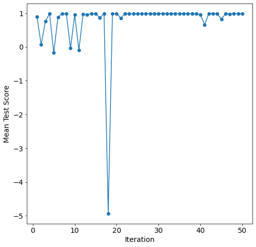
The Bayesian search overall improves performance as it optimizes the neural network hyper-parameters.

Model Post-processing

With the models tuned and the top num_configs_saved saved, we can now pass these models to the PostProcessor for model comparison and analysis. Additionally if you wish to update some hyper-parmeters, a dictionary similar to model initialization can be passed.

new_model_settings = {
    "nn": {"epochs": 200}
}
postprocessor = mai.PostProcessor(
    data=data,
    models_list=[random_search_configs, bayesian_search_configs],
    new_model_settings=new_model_settings,
    yscaler=preprocessor.yscaler,
)

The models can now be output using the metrics function in the PostProcessor. This returns an ordered table with training and testing \(R^2\), mean absolute error (MAE), mean squared error (MSE), and root mean squared error (RMSE). By default these models are ordered by descending test \(R^2\); however, it can also be ordered along other metrics using the sort_by parameter of metrics. For all but the \(R^2\) the data presented is ascending.

postprocessor.metrics()

	Model Types	Parameter Configurations	Train R2	Train MAE	Train MSE	Train RMSE	Test R2	Test MAE	Test MSE	Test RMSE
1	lasso	{'alpha': 0.00011901776919387228}	0.995145	12.540464	314.249861	17.727094	0.994272	13.202008	379.244682	19.474206
2	lasso	{'alpha': 0.00013819863350479427}	0.995136	12.574848	314.874030	17.744690	0.994270	13.232089	379.568911	19.482528
3	lasso	{'alpha': 0.00015471892799623344}	0.995127	12.605704	315.486238	17.761932	0.994266	13.259614	379.928279	19.491749
4	lasso	{'alpha': 0.00015923155092465916}	0.995125	12.614330	315.665474	17.766977	0.994265	13.267455	380.039335	19.494598
0	linear	{'copy_X': True, 'fit_intercept': True, 'n_job...	0.995170	12.363555	312.457800	17.676476	0.994257	13.062255	379.466950	19.479911
5	lasso	{'alpha': 0.00019463957122076609}	0.995102	12.686000	317.250672	17.811532	0.994255	13.333352	381.102729	19.521853
22	nn	{'batch_size': 27, 'learning_rate': 0.00099320...	0.993175	17.183395	532.163538	23.068670	0.991212	19.240779	701.060026	26.477538
25	nn	{'batch_size': 27, 'learning_rate': 0.00097651...	0.992316	18.039954	587.198945	24.232188	0.990606	20.160411	760.834122	27.583222
24	nn	{'batch_size': 27, 'learning_rate': 0.00099716...	0.991723	18.788075	661.885404	25.727134	0.990368	20.187976	808.078463	28.426721
23	nn	{'batch_size': 27, 'learning_rate': 0.00096118...	0.992360	17.678547	571.987472	23.916260	0.990192	20.225215	792.375886	28.149172
21	nn	{'batch_size': 27, 'learning_rate': 0.001, 'mi...	0.989653	20.461923	709.969659	26.645256	0.987723	22.692531	889.640625	29.826844
17	knn	{'leaf_size': 26, 'n_neighbors': 7, 'p': 2, 'w...	1.000000	0.000000	0.000000	0.000000	0.934230	54.810917	5354.475986	73.174285
18	knn	{'leaf_size': 8, 'n_neighbors': 7, 'p': 2, 'we...	1.000000	0.000000	0.000000	0.000000	0.934230	54.810917	5354.475986	73.174285
16	knn	{'leaf_size': 29, 'n_neighbors': 7, 'p': 2, 'w...	1.000000	0.000000	0.000000	0.000000	0.934230	54.810917	5354.475986	73.174285
20	knn	{'leaf_size': 19, 'n_neighbors': 5, 'p': 2, 'w...	1.000000	0.000000	0.000000	0.000000	0.931675	55.902151	5513.439905	74.252541
19	knn	{'leaf_size': 1, 'n_neighbors': 5, 'p': 2, 'we...	1.000000	0.000000	0.000000	0.000000	0.931675	55.902151	5513.439905	74.252541
11	rforest	{'criterion': 'absolute_error', 'max_features'...	0.973803	33.385883	1998.600576	44.705711	0.881174	72.392346	9503.854915	97.487717
12	rforest	{'criterion': 'squared_error', 'max_features':...	0.972705	34.095822	2079.097164	45.597118	0.877348	73.452169	9840.248722	99.198028
13	rforest	{'criterion': 'poisson', 'max_features': None,...	0.947283	47.653228	4028.601943	63.471269	0.875421	74.537864	9940.798642	99.703554
15	rforest	{'criterion': 'squared_error', 'max_features':...	0.934153	53.504930	5008.958815	70.773998	0.866974	77.631052	10684.526665	103.365984
14	rforest	{'criterion': 'poisson', 'max_features': 'sqrt...	0.952741	44.857990	3593.681056	59.947319	0.865804	76.800518	10734.088958	103.605448
7	dtree	{'max_depth': 22, 'max_features': 6, 'min_samp...	0.874288	74.227726	9663.043750	98.300782	0.720513	112.956621	22485.605656	149.952011
8	dtree	{'max_depth': 43, 'max_features': None, 'min_s...	0.874288	74.227726	9663.043750	98.300782	0.720185	113.101494	22565.698611	150.218836
10	dtree	{'max_depth': 49, 'max_features': None, 'min_s...	0.901674	65.365518	7525.509725	86.749696	0.714783	113.714697	22807.587862	151.021813
6	dtree	{'max_depth': 18, 'max_features': 6, 'min_samp...	0.901674	65.365518	7525.509725	86.749696	0.714380	113.285736	22776.112460	150.917568
9	dtree	{'max_depth': 44, 'max_features': 6, 'min_samp...	0.889473	69.575690	8446.504047	91.904864	0.709377	114.846985	23244.619453	152.461862

These results indicate a linear data set as both linear and lasso are the top performing models. nn proves its versitility with close performance to linear and lasso. While the knn models perform adequatly, their training \(R^2\) are equal to 1.0, this indicates an overfit model. Both rforest and dtree overfit to the MIT reactor data set with test \(R^2\) less than or equal to 0.90.

Using the get_params function we can see the parameters (only those subject to tuning) of a model by the name or index in the metrics table. For names given the configuration of that model with the best test \(R^2\) is returned. If no index or name is given then the model with the best test \(R^2\) is given. Here are the tuning configurations of the top model of each model type:

for model in model_settings["models"]:
    print(postprocessor.get_params(model_type=model), "\n")

  Model Types  copy_X  fit_intercept n_jobs   normalize  positive
0      linear    True           True   None  deprecated     False

  Model Types     alpha
0       lasso  0.000119

  Model Types  max_depth  max_features  min_samples_leaf  min_samples_split
0       dtree         22             6                 4                  4

  Model Types  leaf_size  n_neighbors  p   weights
0         knn         29            7  2  distance

  Model Types       criterion  max_features  min_samples_leaf  \
0     rforest  absolute_error             2                 1

   min_samples_split  n_estimators
0                  3           184

  Model Types  batch_size  learning_rate mid_num_node_strategy  num_layers  \
0          nn          27       0.000993                linear           3

   start_num_nodes
0              300

To visualize the performance of these models the diagonal_validation_plot and validation_plot functions can be used to produce diagonal validation and validation plots. Diagonal validation plots show how well the outputs predicted by the model for the training and testing data sets compare to the actual output. A well fit model follows \(y=x\).

models = np.array([["linear", "lasso"], ["dtree", "knn"], ["rforest", "nn"]])
fig, axarr = plt.subplots(models.shape[0], models.shape[1], sharex=True, sharey=True, figsize=(15,20))
for i in range(models.shape[0]):
    for j in range(models.shape[1]):
        plt.sca(axarr[i, j])
        axarr[i, j] = postprocessor.diagonal_validation_plot(model_type=models[i, j])
        axarr[i, j].set_title(models[i, j])

All models display close spread to \(y=x\); however, the lack of performance in dtree and rforest are apparent in the larger spread.

Validation plots show the absolute error of the predicted output relative to the actual outputs of the testing data set. The function can evaluate all output or show just what is given in a list. This list can include column positions in the data set or the output names. For the validation plot below only the A-2, B-8, and C-8 fuel elements are shown.

fig, axarr = plt.subplots(models.shape[0], models.shape[1], figsize=(17,22))

y = ["A-2", "B-8", "C-8"]
for i in range(models.shape[0]):
    for j in range(models.shape[1]):
        plt.sca(axarr[i, j])
        axarr[i, j] = postprocessor.validation_plot(model_type=models[i, j], y=y)
        axarr[i, j].set_title(models[i, j])
        axarr[i, j].get_legend().remove()

fig.legend(y, loc="upper center", ncol=4)

The diagonal validation and validation plots agree with the performance metrics. The errors of rforest or dtree is higher than linear, lasso, nn, and knn.

To further understand the behavior of the top neural network configurations we can plot the learning curve. Here the top neural network learning curve is shown but, similar to the diagonal_validation_plot and validation_plot functions, nn_learning_plot shows the neural network based on the index in metrics or, if no index is provided, the one with the best test \(R^2\).

fig, ax = plt.subplots(figsize=(8,8))
ax = postprocessor.nn_learning_plot()

The validation curve is below the training for the each epoch; therefore, the top neural networks configuration is not overfit to the training data.

Finally, using the linear regression model we can generate a predicted power for each fuel element given the control blade heights.

def plot_mitr(model, x, yscaler=None):
    pos=[(400,330), (465,230), (500,300), (395,400), (320,400), (285,255), (318,193),
         (500,165), (535,230), (575,295), (535,360), (500,430), (430,465), (355,465),
         (280,465), (240,400), (205,335), (210,255), (243,193), (280,130), (355,130),
         (430,130), (393,193), (460,360), (280,335), (400,265), (340,295)]

    Ynn=model.predict(np.array([x,]))
    if yscaler:
        Ynn=yscaler.inverse_transform(Ynn)
    Ynn=Ynn.flatten().tolist()

    image = cv2.imread("./supporting/mitr.png")
    for i in range(len(pos)):
        if i==0:
            image=cv2.putText(img=np.copy(image), text=str(int(Ynn[i])), org=pos[i], fontFace=1, fontScale=1.1, color=(0,0,0))
        if i in [1,2,3,4,5,6]:
            image=cv2.putText(img=np.copy(image), text=str(int(Ynn[i])), org=pos[i], fontFace=1, fontScale=1.1, color=(0,0,255))
        if i in list(range(7,22)):
            image=cv2.putText(img=np.copy(image), text=str(int(Ynn[i])), org=pos[i], fontFace=1, fontScale=1.1, color=(0, 100, 0))
        if i in list(range(22,28)):
            image=cv2.putText(img=np.copy(image), text=str('Empty'), org=pos[i], fontFace=1, fontScale=1.1, color=(233, 150, 122))
    plt.figure(figsize=(12, 12))
    plt.imshow(image)
    plt.axis('off')

x=[0.75266553, 0.90280633, 0.00539489, 0.25308624, 0.57678792, 0.77792903]

plot_mitr(postprocessor.get_model(model_type="linear"), x, preprocessor.yscaler)

References

1. 13. 1. RADAIDEH, K. DU, P. SEURIN, D. SEYLER, X. GU, H. WANG, and K. SHIRVAN, “NEORL: NeuroEvolution Optimization with Reinforcement Learning,” CoRR, abs/2112.07057 (2021).