Reactor Physics

Inputs: 2-group homogenized cross sections (HXS) (\(cm^{-1}\))

• FissionFast: \(\nu\Sigma_f^1\)

• CaptureFast: \(\Sigma_a^1\)

• FissionThermal: \(\nu\Sigma_f^2\)

• CaptureThermal: \(\Sigma_a^2\)

• Scatter12: \(\Sigma_s^{1 \rightarrow 2}\)

• Scatter11: \(\Sigma_s^{1 \rightarrow 1}\)

• Scatter21: \(\Sigma_s^{2 \rightarrow 1}\)

• Scatter22: \(\Sigma_s^{2 \rightarrow 2}\)

Outputs

• k: Neutron multipulcation factor

This data set consists of 1000 observations with 8 inputs and 1 output. The data is taken from [1], a sensitivity analysis using the Shapley effect. The geometry of the problem is a pressurized water reactor (PWR) lattice based on the BEAVRS benchmark. The lattice is a \(17 \times 17\) PWR with \(264~UO_2\) fuel rods, 24 guide tubes, and one instrumentation tube. The lattice utilizes quarter symmetry in TRITON and is depleted to \(50~GWD/MTU\). To construct the data set, a two-step process was used: (1) the uncertainty in the fundamental microscopic XS data was propagated, and (2) these XSs were collapsed into a 2-group form using the following equation

\begin{equation} \Sigma_x^g = \frac{\int_{\Delta E_g}dE \int_V \Sigma_{x,m}(E) \phi(r,E,t) dV}{\int_{\Delta E_g}dE\int_V\phi(r,E,t)dV}. \end{equation}

The Sampler module in SCALE was used for uncertainty propagation, and the 56-group XS and covariance libraries were used in TRITON to create 56-group HXSs using the above equation. These HXSs are then collapsed into a 2-group library. 1000 random samples were taken from the Sampler.

import pyMAISE as mai
import time
import pandas as pd
import numpy as np
import matplotlib.pyplot as plt
from matplotlib.gridspec import GridSpec
from scipy.stats import uniform, randint
from sklearn.model_selection import ShuffleSplit

# Plot settings
matplotlib_settings = {
    "font.size": 14,
    "legend.fontsize": 12,
}
plt.rcParams.update(**matplotlib_settings)

pyMAISE Initialization

pyMAISE will be initialized with the following global settings:

• verbosity: 0 \(\rightarrow\) pyMAISE prints no outputs,

• random_state: None \(\rightarrow\) no random seed is set,

• test_size: 0.3 \(\rightarrow\) 30% of the data is used for testing,

• num_configs_saved: 5 \(\rightarrow\) the top 5 hyper-parameter configurations are saved for each model.

We can load the reactor physics pre-processor by load_xs().

global_settings = mai.settings.init()
preprocessor = mai.load_xs()

The data consists of 8 inputs:

preprocessor.inputs.head()

	FissionFast	CaptureFast	FissionThermal	CaptureThermal	Scatter12	Scatter11	Scatter21	Scatter22
0	0.006446	0.009248	0.130007	0.080836	0.014973	0.482483	0.001506	1.12546
1	0.006359	0.009347	0.128811	0.081048	0.015363	0.490558	0.001497	1.12616
2	0.006467	0.009253	0.129465	0.080762	0.015198	0.486784	0.001493	1.12423
3	0.006479	0.009258	0.130903	0.081478	0.015345	0.492895	0.001516	1.13075
4	0.006431	0.009248	0.129757	0.081129	0.015216	0.488249	0.001506	1.12731

and one output with 1000 data points:

preprocessor.outputs.head()

	k
0	1.256376
1	1.241534
2	1.256988
3	1.261442
4	1.253744

To get a better idea of the data we can create a corrilation matrix using the correlation_matrix() function.

fig, ax = plt.subplots(figsize=(15,10))
fig, ax = preprocessor.correlation_matrix(fig=fig, ax=ax, colorbar=False, annotations=True)

There is a positive correlation between k with FissionFast and FissionThermal.

The last step of initialization is scaling, we will min-max scale this data.

data = preprocessor.min_max_scale()

Model Initialization

As this data set had a 1-dimensional output, we will hyper-parameter 7 models:

• Linear regression: linear,

• Lasso regression: lasso,

• Support vector regression: svr,

• Decision tree regression: dtree,

• Random forest regression: rforest,

• K-nearest neighbors regression: knn,

• Sequential Dense Neural Networks: nn.

All the classical models are initialized with the Scikit-learn defaults; however, the neural networks require some paramter definitions for the layers, optimizer, and training.

model_settings = {
    "models": ["linear", "lasso", "dtree", "svr", "knn", "rforest", "nn"],
    "nn": {
        # Sequential
        "num_layers": 4,
        "dropout": True,
        "rate": 0.5,
        "validation_split": 0.15,
        "loss": "mean_absolute_error",
        "metrics": ["mean_absolute_error"],
        "batch_size": 8,
        "epochs": 50,
        "warm_start": True,
        "jit_compile": False,
        # Starting Layer
        "start_num_nodes": 100,
        "start_kernel_initializer": "normal",
        "start_activation": "relu",
        "input_dim": preprocessor.inputs.shape[1], # Number of inputs
        # Middle Layers
        "mid_num_node_strategy": "linear", # Middle layer nodes vary linearly from 'start_num_nodes' to 'end_num_nodes'
        "mid_kernel_initializer": "normal",
        "mid_activation": "relu",
        # Ending Layer
        "end_num_nodes": preprocessor.outputs.shape[1], # Number of outputs
        "end_activation": "linear",
        "end_kernel_initializer": "normal",
        # Optimizer
        "optimizer": "adam",
        "learning_rate": 5e-4,
    },
}
tuning = mai.Tuning(data=data, model_settings=model_settings)

Hyper-parameter Tuning

They hyper-parameter tuning spaces are defined below. We use random search for the classical models as their training is quick and random search can cover a large parameter space. Bayesian search is used for the neural networks as their training is more computationally expensive. Both search methods use 5-fold cross-validation to mitigate bias from the training data. We train 300 classical models from random search and 50 iterations of Bayesian search for neural networks.

random_search_spaces = {
    "lasso": {
        "alpha": uniform(loc=0.0001, scale=0.0099), # 0.0001 - 0.01
    },
    "dtree": {
        "max_depth": randint(low=5, high=50), # 5 - 50
        "max_features": [None, "sqrt", "log2", 2, 4, 6],
        "min_samples_split": randint(low=2, high=20), # 2 - 20
        "min_samples_leaf": randint(low=1, high=20), # 1 - 20
    },
    "svr": {
        "kernel": ["linear", "poly", "rbf", "sigmoid"],
        "degree": randint(low=1, high=5),
        "gamma": ["scale", "auto"],
    },
    "rforest": {
        "n_estimators": randint(low=50, high=200), # 50 - 200
        "criterion": ["squared_error", "absolute_error", "poisson"],
        "min_samples_split": randint(low=2, high=20), # 2 - 20
        "min_samples_leaf": randint(low=1, high=20), # 1 - 20
        "max_features": [None, "sqrt", "log2", 2, 4, 6],
    },
    "knn": {
        "n_neighbors": randint(low=1, high=20), # 1 - 20
        "weights": ["uniform", "distance"],
        "leaf_size": randint(low=1, high=30), # 1 - 30
        "p": randint(low=1, high=10), # 1 - 10
    },
}
bayesian_search_spaces = {
    "nn": {
        "mid_num_node_strategy": ["constant", "linear"],
        "batch_size": [8, 64],
        "learning_rate": [1e-5, 0.001],
        "num_layers": [2, 6],
        "start_num_nodes": [25, 300],
    },
}

start = time.time()
random_search_configs = tuning.random_search(
    param_spaces=random_search_spaces,
    models=["linear"] + list(random_search_spaces.keys()),
    n_iter=300,
    cv=ShuffleSplit(n_splits=5, test_size=0.25, random_state=global_settings.random_state),
)
bayesian_search_configs = tuning.bayesian_search(
    param_spaces=bayesian_search_spaces,
    models=bayesian_search_spaces.keys(),
    n_iter=50,
    cv=5,
)
stop = time.time()
print("Hyper-parameter tuning took " + str((stop - start) / 60) + " minutes to process.")

Hyper-parameter tuning search space was not provided for linear, doing manual fit
Hyper-parameter tuning took 76.84055530627569 minutes to process.

We can see the Bayesian search hyper-parameter optimization in the convergence plot.

fig, ax = plt.subplots(figsize=(8,8))
ax = tuning.convergence_plot(model_types="nn")

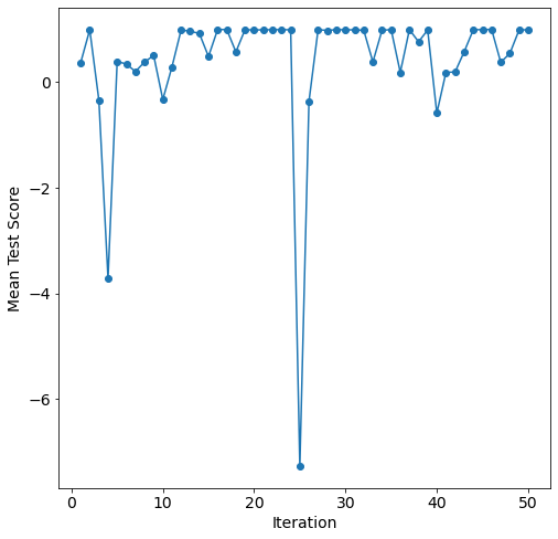
It appears to converge at around the 30th iteration.

Model Post-processing

With the top num_configs_saved, we can pass these parameter configurations to the PostProcessor for model comparison and analysis. For nn we define the epochs parameter to be 200 for better performance.

new_model_settings = {
    "nn": {"epochs": 200}
}
postprocessor = mai.PostProcessor(
    data=data,
    models_list=[random_search_configs, bayesian_search_configs],
    new_model_settings=new_model_settings,
    yscaler=preprocessor.yscaler,
)

To compare the performance of these models we will compute 4 metrics for both the training and testing data:

• mean squared error MSE \(=\frac{1}{n}\sum^n_{i = 1}(y_i - \hat{y_i})^2\),

• root mean squared error RMSE \(=\sqrt{\frac{1}{n}\sum^n_{i = 1}(y_i - \hat{y_i})^2}\),

• mean absolute error MAE = \(=\frac{1}{n}\sum^n_{i = 1}|y_i - \hat{y_i}|\),

• and r-squared R2 \(=1 - \frac{\sum^n_{i = 1}(y_i - \hat{y_i})^2}{\sum^n_{i = 1}(y_i - \bar{y_i})^2}\),

where \(y\) is the actual outcome, \(\bar{y}\) is the average outcome, \(\bar{y}\) is the model predicted outcome, and \(n\) is the number of observations.

postprocessor.metrics()

	Model Types	Parameter Configurations	Train R2	Train MAE	Train MSE	Train RMSE	Test R2	Test MAE	Test MSE	Test RMSE
0	linear	{'copy_X': True, 'fit_intercept': True, 'n_job...	0.999922	0.000046	4.393845e-09	0.000066	0.999943	0.000039	2.718327e-09	0.000052
1	lasso	{'alpha': 0.00014534810804869164}	0.999539	0.000129	2.586986e-08	0.000161	0.999493	0.000120	2.433484e-08	0.000156
2	lasso	{'alpha': 0.00014581414227680752}	0.999537	0.000129	2.600405e-08	0.000161	0.999490	0.000121	2.446925e-08	0.000156
3	lasso	{'alpha': 0.00023820902388072067}	0.998912	0.000200	6.109612e-08	0.000247	0.998760	0.000190	5.950986e-08	0.000244
26	nn	{'batch_size': 8, 'learning_rate': 0.000895759...	0.998786	0.000184	6.819188e-08	0.000261	0.998717	0.000172	6.160771e-08	0.000248
4	lasso	{'alpha': 0.00024356169338852368}	0.998867	0.000204	6.364692e-08	0.000252	0.998708	0.000195	6.205178e-08	0.000249
30	nn	{'batch_size': 63, 'learning_rate': 0.00095445...	0.998932	0.000170	5.998744e-08	0.000245	0.998597	0.000168	6.734411e-08	0.000260
5	lasso	{'alpha': 0.000256506780154024}	0.998753	0.000214	7.005040e-08	0.000265	0.998575	0.000204	6.843109e-08	0.000262
29	nn	{'batch_size': 8, 'learning_rate': 0.000913485...	0.997883	0.000263	1.188860e-07	0.000345	0.997939	0.000240	9.895146e-08	0.000315
27	nn	{'batch_size': 8, 'learning_rate': 0.000902521...	0.998082	0.000287	1.076765e-07	0.000328	0.997848	0.000280	1.033429e-07	0.000321
28	nn	{'batch_size': 8, 'learning_rate': 0.000888746...	0.997937	0.000304	1.158278e-07	0.000340	0.997711	0.000295	1.099015e-07	0.000332
15	svr	{'degree': 1, 'gamma': 'scale', 'kernel': 'lin...	0.935440	0.001539	3.625248e-06	0.001904	0.922994	0.001510	3.697144e-06	0.001923
11	svr	{'degree': 3, 'gamma': 'scale', 'kernel': 'lin...	0.935440	0.001539	3.625248e-06	0.001904	0.922994	0.001510	3.697144e-06	0.001923
12	svr	{'degree': 3, 'gamma': 'scale', 'kernel': 'lin...	0.935440	0.001539	3.625248e-06	0.001904	0.922994	0.001510	3.697144e-06	0.001923
13	svr	{'degree': 1, 'gamma': 'auto', 'kernel': 'line...	0.935440	0.001539	3.625248e-06	0.001904	0.922994	0.001510	3.697144e-06	0.001923
14	svr	{'degree': 4, 'gamma': 'scale', 'kernel': 'lin...	0.935440	0.001539	3.625248e-06	0.001904	0.922994	0.001510	3.697144e-06	0.001923
17	rforest	{'criterion': 'poisson', 'max_features': None,...	0.987259	0.000657	7.154440e-07	0.000846	0.914143	0.001549	4.122079e-06	0.002030
16	rforest	{'criterion': 'poisson', 'max_features': 6, 'm...	0.981090	0.000787	1.061829e-06	0.001030	0.911553	0.001549	4.246429e-06	0.002061
19	rforest	{'criterion': 'squared_error', 'max_features':...	0.978982	0.000841	1.180233e-06	0.001086	0.908445	0.001591	4.395637e-06	0.002097
18	rforest	{'criterion': 'absolute_error', 'max_features'...	0.975491	0.000906	1.376239e-06	0.001173	0.907988	0.001590	4.417570e-06	0.002102
20	rforest	{'criterion': 'poisson', 'max_features': 6, 'm...	0.966660	0.001047	1.872149e-06	0.001368	0.896801	0.001666	4.954699e-06	0.002226
22	knn	{'leaf_size': 20, 'n_neighbors': 6, 'p': 4, 'w...	1.000000	0.000000	0.000000e+00	0.000000	0.868669	0.001835	6.305312e-06	0.002511
21	knn	{'leaf_size': 13, 'n_neighbors': 6, 'p': 5, 'w...	1.000000	0.000000	0.000000e+00	0.000000	0.867161	0.001838	6.377698e-06	0.002525
24	knn	{'leaf_size': 6, 'n_neighbors': 5, 'p': 4, 'we...	1.000000	0.000000	0.000000e+00	0.000000	0.864873	0.001826	6.487579e-06	0.002547
23	knn	{'leaf_size': 28, 'n_neighbors': 5, 'p': 3, 'w...	1.000000	0.000000	0.000000e+00	0.000000	0.861551	0.001847	6.647085e-06	0.002578
25	knn	{'leaf_size': 17, 'n_neighbors': 4, 'p': 3, 'w...	1.000000	0.000000	0.000000e+00	0.000000	0.860524	0.001908	6.696392e-06	0.002588
9	dtree	{'max_depth': 10, 'max_features': 6, 'min_samp...	0.908292	0.001718	5.149704e-06	0.002269	0.793738	0.002487	9.902836e-06	0.003147
7	dtree	{'max_depth': 43, 'max_features': 6, 'min_samp...	0.933476	0.001472	3.735503e-06	0.001933	0.770848	0.002643	1.100178e-05	0.003317
10	dtree	{'max_depth': 16, 'max_features': 6, 'min_samp...	0.979714	0.000790	1.139137e-06	0.001067	0.762098	0.002733	1.142190e-05	0.003380
6	dtree	{'max_depth': 19, 'max_features': 6, 'min_samp...	0.924182	0.001582	4.257388e-06	0.002063	0.750213	0.002679	1.199250e-05	0.003463
8	dtree	{'max_depth': 16, 'max_features': 4, 'min_samp...	0.925655	0.001572	4.174666e-06	0.002043	0.720919	0.002856	1.339895e-05	0.003660

The top performing models are linear, lasso, nn, and svr; however, rforest is above 0.90 test r-squared. Given the linear models are the most performant models we can safely saw this data set is linear. We can see that knn and dtree are overfit given the difference between Train R2 and Test R2.

We can see the hyper-parameter configurations of each top Test R2 model with the get_params function.

for model in model_settings["models"]:
    print(postprocessor.get_params(model_type=model), "\n")

  Model Types  copy_X  fit_intercept n_jobs  positive
0      linear    True           True   None     False

  Model Types     alpha
0       lasso  0.000145

  Model Types  max_depth  max_features  min_samples_leaf  min_samples_split
0       dtree         10             6                 7                  6

  Model Types  degree  gamma  kernel
0         svr       3  scale  linear

  Model Types  leaf_size  n_neighbors  p   weights
0         knn         20            6  4  distance

  Model Types criterion max_features  min_samples_leaf  min_samples_split  \
0     rforest   poisson         None                 1                  3

   n_estimators
0           194

  Model Types  batch_size  learning_rate mid_num_node_strategy  num_layers  \
0          nn           8       0.000896              constant           2

   start_num_nodes
0              300

We can better visualize the performance of each model with diagonal validation plots.

models = np.array([["linear", "lasso"], ["dtree", "svr"], ["knn", "rforest"], ["nn", None]])

fig = plt.figure(constrained_layout=fig, figsize=(10,20))
gs = GridSpec(models.shape[0], models.shape[1], figure=fig)
for i in range(models.shape[0] - 1):
    for j in range(models.shape[1]):
        if models[i, j] != None:
            ax = fig.add_subplot(gs[i, j])
            ax = postprocessor.diagonal_validation_plot(model_type=models[i, j])
            ax.set_title(models[i, j])
ax = fig.add_subplot(gs[-1, :])
ax = postprocessor.diagonal_validation_plot(model_type=models[-1, 0])
_ = ax.set_title(models[-1, 0])

linear, lasso, and nn are tightly spread near \(y = x\). The overfit of knn is apparent in the difference in spread of training compared to testing.

Validation plots tell us a similar story.

fig = plt.figure(constrained_layout=fig, figsize=(10,20))
gs = GridSpec(models.shape[0], models.shape[1], figure=fig)
for i in range(models.shape[0] - 1):
    for j in range(models.shape[1]):
        if models[i, j] != None:
            ax = fig.add_subplot(gs[i, j])
            ax = postprocessor.validation_plot(model_type=models[i, j])
            ax.set_title(models[i, j])
ax = fig.add_subplot(gs[-1, :])
ax = postprocessor.validation_plot(model_type=models[-1, 0])
_ = ax.set_title(models[-1, 0])

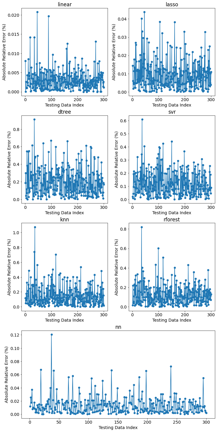
linear, lasso, and nn have all testing relative errors less than 0.10.

Finally, we can see if nn was overfit in learning curves.

fig, ax = plt.subplots(figsize=(8,8))
ax = postprocessor.nn_learning_plot()

The validation curve is below the training curve; therefore, this nn was not overfit.

References

1. 13. 1. Radaideh, S. Surani, D. O’Grady, and T. Kozlowski, “Shapley effect application for variance-based sensitivity analysis of the few-group cross-sections,” Annals of Nuclear Energy, vol. 129, pp. 264–279, 2019.