BWR Micro Core

Inputs

• PSZ: Fuel bundle region Power Shaping Zone (PSZ).

• DOM: Fuel bundle region Dominant zone (DOM).

• vanA: Fuel bundle region vanishing zone A (VANA).

• vanB: Fuel bundle region vanishing zone B (VANB)

• subcool: Represents moderator inlet conditions. Core inlet subcooling interpreted to be at the steam dome pressure (i.e., not core-averaged pressure). The input value for subcooling will automatically be increased to account for this fact. (Btu/lb)?

• CRD: Defines the position of all control rod groups (banks).

• flow_rate: Defines essential global design data for rated coolant mass flux for the active core, \(\frac{kg}{(cm^{2}-hr)}\). Coolant mass flux equals active core flow divided by core cross-section area. Core cross-section area is DXA 2 times the number of assemblies.

• power_density: Defines essential global design data for rated power density using cold dimensions, \((\frac{kw}{liter})\).

• VFNGAP: Defines the ratio of narrow water gap width to the sum of the narrow and wide water gap widths.

Output

• K-eff: Reactivity coefficient k-effective, the effective neutron multiplication factor.

• Max3Pin: Maximum planar-averaged pin power peaking factor.

• Max4Pin: maximum pin-power peaking factor, \(F_{q}\), (which includes axial intranodal peaking).

• F-delta-H: Ratio of max-to-average enthalpy rise in a channel.

• Max-Fxy: Maximum radial pin-power peaking factor.

  The data set consists of 2000 data points with 9 inputs and 5 outputs. This data set was constructed through uniform and normal sampling of the 9 input parameters for a boiling water reactor (BWR) micro-core. These samples were then used to solve for reactor characteristic changes in heat distribution and neutron flux. This BWR micro-core consists of 4 radially and axially heterogenous assemblies of the same type constructed in a 2x2 grid with a control blade placed in the center. A single assembly composition can be seen in the figure below. A single assembly was brocken into seven zones where each zones 2D radial cross sectional information was constructed using CASMO-4. These cross sectional libraries were then processed through CMSLINK for SIMULATE-3 to interpret. The core geometry and physics was implemented and modeled using SIMULATE-3.

import pyMAISE as mai
import time
import pandas as pd
import numpy as np
import matplotlib.pyplot as plt
from matplotlib.gridspec import GridSpec
from scipy.stats import uniform, randint
from sklearn.model_selection import ShuffleSplit

# Plot settings
matplotlib_settings = {
    "font.size": 14,
    "legend.fontsize": 12,
}
plt.rcParams.update(**matplotlib_settings)

pyMAISE Initialization

Starting any pyMAISE job requires initialization, this includes the definition of global settings used throughout pyMAISE. For this problem the pyMAISE defaults are used:

• verbosity: 0 \(\rightarrow\) pyMAISE prints no outputs,

• random_state: None \(\rightarrow\) No random seed is set,

• test_size: 0.3 \(\rightarrow\) 30% of the data is used for testing,

• num_configs_saved: 5 \(\rightarrow\) The top 5 hyper-parameter configurations are saved for each model.

The settings are initialized and the heat conduction preprocessor specific to this data set is retrieved.

global_settings = mai.settings.init()
preprocessor = mai.load_BWR()

The BWR micro reactor data set has 9 inputs

preprocessor.inputs.head()

	PSZ	DOM	vanA	vanB	subcool	CRD	flow_rate	power_density	VFNGAP
0	120.334	216.336	338.763	332.827	24.168	15	250.161	66.250	0.222
1	137.906	198.764	349.531	322.059	22.435	30	253.792	66.044	0.393
2	131.235	205.435	317.283	354.307	24.234	16	255.631	65.839	0.432
3	127.169	209.501	303.856	367.734	27.501	47	252.619	63.828	0.360
4	113.670	223.000	306.145	365.445	22.188	8	256.789	64.326	0.442

and 5 outputs with 2000 samples

preprocessor.outputs.head()

	K-eff	Max3Pin	Max4Pin	F-delta-H	Max-Fxy
0	0.95455	5.105	5.303	1.861	1.899
1	0.98576	2.839	2.904	1.436	1.816
2	0.95237	5.161	5.430	1.846	1.903
3	0.99724	2.500	2.575	1.246	1.584
4	0.87466	6.259	6.635	1.580	1.900

To better understand the data here is a correlation matrix of the data.

fig, ax = plt.subplots(figsize=(15,10))
fig, ax = preprocessor.correlation_matrix(fig=fig, ax=ax, colorbar=False, annotations=True)

As expected there is a strong negative correlation between control rod position (CRD) and the peaking factors. There is also a strong positive correlation between control rod position and k effective.

Prior to model training the data is min-max scaled to make each feature’s effect size is comparable. Additionally, this can improve the performance of some models.

data = preprocessor.min_max_scale()

Model Initialization

Given this data set has a multi-dimensional output we will compare the performance of 7 machine learning (ML) models:

• Linear regression: linear,

• Lasso regression: lasso,

• Decision tree regression: dtree,

• Random forest regression: rforest,

• K-nearest neighbors regression: knn,

• Sequential dense neural networks: nn.

For hyper-parameter tuning each model must be initialized. We will use the Scikit-learn defaults for the classical ML models (linear, lasso, dtree, rforest, and knn); therefore, they are only specified in the models parameter of the model_settings dictionary. However, we must specify many parameters for the nn model that define the layers, optimizer, and training.

model_settings = {
    "models": ["linear", "lasso", "dtree", "knn", "rforest", "nn"],
    "nn": {
        # Sequential
        "num_layers": 4,
        "dropout": True,
        "rate": 0.5,
        "validation_split": 0.15,
        "loss": "mean_absolute_error",
        "metrics": ["mean_absolute_error"],
        "batch_size": 8,
        "epochs": 50,
        "warm_start": True,
        "jit_compile": False,
        # Starting Layer
        "start_num_nodes": 100,
        "start_kernel_initializer": "normal",
        "start_activation": "relu",
        "input_dim": preprocessor.inputs.shape[1], # Number of inputs
        # Middle Layers
        "mid_num_node_strategy": "linear", # Middle layer nodes vary linearly from 'start_num_nodes' to 'end_num_nodes'
        "mid_kernel_initializer": "normal",
        "mid_activation": "relu",
        # Ending Layer
        "end_num_nodes": preprocessor.outputs.shape[1], # Number of outputs
        "end_activation": "linear",
        "end_kernel_initializer": "normal",
        # Optimizer
        "optimizer": "adam",
        "learning_rate": 5e-4,
    },
}
tuning = mai.Tuning(data=data, model_settings=model_settings)

Hyper-parameter Tuning

While three hyper-parameter tuning functions are supported (grid_search, random_search, and bayesian_search), random_search and bayesian_search are used for the classical ML and nn models, respectively. random_search randomly samples a defined parameter space and the number of models generated is easily defined. A large number of classical models are generated through random_search as they are relatively quick to train. However, the prohibative time required to train neural networks makes bayesian_search more appealing as the search converges to the optimal hyper-parameters in relatively few iterations. The hyper-parameter search spaces are outlined below, many with Scipy uniform distributions. Cross validation is used in both search methods to eliminate bias from the data set.

random_search_spaces = {
    "lasso": {
        "alpha": uniform(loc=0.0001, scale=0.0099), # 0.0001 - 0.01
    },
    "dtree": {
        "max_depth": randint(low=5, high=50), # 5 - 50
        "max_features": [None, "sqrt", "log2", 2, 4, 6],
        "min_samples_split": randint(low=2, high=20), # 2 - 20
        "min_samples_leaf": randint(low=1, high=20), # 1 - 20
    },
    "rforest": {
        "n_estimators": randint(low=50, high=200), # 50 - 200
        "criterion": ["squared_error", "absolute_error", "poisson"],
        "min_samples_split": randint(low=2, high=20), # 2 - 20
        "min_samples_leaf": randint(low=1, high=20), # 1 - 20
        "max_features": [None, "sqrt", "log2", 2, 4, 6],
    },
    "knn": {
        "n_neighbors": randint(low=1, high=20), # 1 - 20
        "weights": ["uniform", "distance"],
        "leaf_size": randint(low=1, high=30), # 1 - 30
        "p": randint(low=1, high=10), # 1 - 10
    },
}
bayesian_search_spaces = {
    "nn": {
        "mid_num_node_strategy": ["constant", "linear"],
        "dropout": [True, False],
        "batch_size": [8, 64],
        "learning_rate": [1e-5, 0.01],
        "num_layers": [2, 8],
        "start_num_nodes": [25, 500],
    },
}

start = time.time()
random_search_configs = tuning.random_search(
    param_spaces=random_search_spaces,
    models=["linear"] + list(random_search_spaces.keys()),
    n_iter=300,
    cv=ShuffleSplit(n_splits=5, test_size=0.25, random_state=global_settings.random_state),
)
bayesian_search_configs = tuning.bayesian_search(
    param_spaces=bayesian_search_spaces,
    models=bayesian_search_spaces.keys(),
    n_iter=50,
    cv=5,
)
stop = time.time()
print("Hyper-parameter tuning took " + str((stop - start) / 60) + " minutes to process.")

Hyper-parameter tuning search space was not provided for linear, doing manual fit
Hyper-parameter tuning took 86.78759005467097 minutes to process.

With the conclusion of training we can see training results for each iteration using the convergence_plot function. For example here is Bayesian search of neural networks:

fig, ax = plt.subplots(figsize=(8,8))
ax = tuning.convergence_plot(model_types="nn")

Fewer than 30 iterations were required to converge to the optimal parameter configurations.

Model Post-processing

With the models tuned and the top num_configs_saved saved, we can now pass these models to the PostProcessor for model comparison and analysis. We will increase the epochs of the nn models for better performance.

new_model_settings = {
    "nn": {"epochs": 200}
}
postprocessor = mai.PostProcessor(
    data=data,
    models_list=[random_search_configs, bayesian_search_configs],
    new_model_settings=new_model_settings,
    yscaler=preprocessor.yscaler,
)

To compare the performance of these models we will compute 4 metrics for both the training and testing data:

• mean squared error MSE \(=\frac{1}{n}\sum^n_{i = 1}(y_i - \hat{y_i})^2\),

• root mean squared error RMSE \(=\sqrt{\frac{1}{n}\sum^n_{i = 1}(y_i - \hat{y_i})^2}\),

• mean absolute error MAE = \(=\frac{1}{n}\sum^n_{i = 1}|y_i - \hat{y_i}|\),

• and r-squared R2 \(=1 - \frac{\sum^n_{i = 1}(y_i - \hat{y_i})^2}{\sum^n_{i = 1}(y_i - \bar{y_i})^2}\),

where \(y\) is the actual outcome, \(\bar{y}\) is the average outcome, \(\hat{y}\) is the model predicted outcome, and \(n\) is the number of observations. The averaged performance metrics are shown below.

postprocessor.metrics()

	Model Types	Parameter Configurations	Train R2	Train MAE	Train MSE	Train RMSE	Test R2	Test MAE	Test MSE	Test RMSE
10	dtree	{'max_depth': 10, 'max_features': None, 'min_s...	0.990065	0.029325	0.007171	0.084683	0.968441	0.056375	0.041258	0.203120
6	dtree	{'max_depth': 23, 'max_features': None, 'min_s...	0.989088	0.030553	0.007748	0.088024	0.967995	0.057324	0.041841	0.204551
7	dtree	{'max_depth': 20, 'max_features': None, 'min_s...	0.988778	0.031133	0.008408	0.091693	0.967823	0.057460	0.042727	0.206706
8	dtree	{'max_depth': 37, 'max_features': None, 'min_s...	0.994997	0.020181	0.003496	0.059128	0.967457	0.056391	0.044830	0.211730
9	dtree	{'max_depth': 24, 'max_features': None, 'min_s...	0.994997	0.020181	0.003496	0.059128	0.967416	0.056598	0.045090	0.212344
11	rforest	{'criterion': 'squared_error', 'max_features':...	0.990724	0.028921	0.007129	0.084435	0.966929	0.054329	0.039736	0.199339
14	rforest	{'criterion': 'squared_error', 'max_features':...	0.987777	0.034477	0.010192	0.100958	0.965517	0.057322	0.041762	0.204357
15	rforest	{'criterion': 'squared_error', 'max_features':...	0.989018	0.032604	0.009257	0.096213	0.965015	0.056036	0.042186	0.205393
12	rforest	{'criterion': 'squared_error', 'max_features':...	0.995220	0.020042	0.004100	0.064031	0.963209	0.053987	0.041549	0.203836
13	rforest	{'criterion': 'poisson', 'max_features': None,...	0.986839	0.034163	0.010585	0.102883	0.962634	0.057911	0.042445	0.206021
22	nn	{'batch_size': 63, 'dropout': 0, 'learning_rat...	0.849404	0.038940	0.015814	0.125754	0.839503	0.049517	0.030795	0.175485
21	nn	{'batch_size': 64, 'dropout': 0, 'learning_rat...	0.843258	0.074322	0.070390	0.265312	0.829471	0.085022	0.097204	0.311775
25	nn	{'batch_size': 35, 'dropout': 0, 'learning_rat...	0.841635	0.072168	0.071638	0.267653	0.828849	0.083265	0.092309	0.303824
24	nn	{'batch_size': 39, 'dropout': 0, 'learning_rat...	0.838570	0.078399	0.077393	0.278196	0.823431	0.090397	0.104874	0.323843
23	nn	{'batch_size': 33, 'dropout': 0, 'learning_rat...	0.839829	0.075223	0.068186	0.261125	0.822959	0.087430	0.098102	0.313213
17	knn	{'leaf_size': 5, 'n_neighbors': 12, 'p': 2, 'w...	1.000000	0.000000	0.000000	0.000000	0.723578	0.169887	0.167618	0.409412
16	knn	{'leaf_size': 1, 'n_neighbors': 7, 'p': 2, 'we...	1.000000	0.000000	0.000000	0.000000	0.722235	0.170336	0.177406	0.421195
18	knn	{'leaf_size': 21, 'n_neighbors': 13, 'p': 2, '...	1.000000	0.000000	0.000000	0.000000	0.721635	0.171167	0.166673	0.408256
19	knn	{'leaf_size': 13, 'n_neighbors': 10, 'p': 3, '...	1.000000	0.000000	0.000000	0.000000	0.720650	0.166312	0.165330	0.406607
20	knn	{'leaf_size': 9, 'n_neighbors': 11, 'p': 3, 'w...	1.000000	0.000000	0.000000	0.000000	0.719483	0.167297	0.164656	0.405778
5	lasso	{'alpha': 0.0006083967482002474}	0.624080	0.229783	0.172287	0.415075	0.623737	0.225957	0.172125	0.414880
2	lasso	{'alpha': 0.0005105108899887478}	0.624375	0.229615	0.172168	0.414932	0.623201	0.225909	0.172257	0.415039
1	lasso	{'alpha': 0.0004860326387070249}	0.624456	0.229575	0.172142	0.414900	0.623055	0.225901	0.172293	0.415082
3	lasso	{'alpha': 0.0004237707539178678}	0.624647	0.229474	0.172073	0.414817	0.622669	0.225864	0.172369	0.415173
4	lasso	{'alpha': 0.0004107875281458962}	0.624686	0.229448	0.172054	0.414794	0.622591	0.225836	0.172368	0.415172
0	linear	{'copy_X': True, 'fit_intercept': True, 'n_job...	0.626111	0.228993	0.171624	0.414275	0.618908	0.225415	0.172057	0.414798

Given the top performing models are decission tree (dtree) and random forest (rforest) this data set’s outputs are non-linear with their inputs. nn performed well, but not amazing. Further analysis will be done later to see which outputs metric brought the values down when averaged. Performance quickly drops off with linear, lasso, and knn. We can look specifically at the performance for each output:

postprocessor.metrics(y="K-eff")

	Model Types	Parameter Configurations	Train R2	Train MAE	Train MSE	Train RMSE	Test R2	Test MAE	Test MSE	Test RMSE
22	nn	{'batch_size': 63, 'dropout': 0, 'learning_rat...	0.992924	0.004380	0.000055	0.007411	0.990673	0.004628	0.000076	0.008734
11	rforest	{'criterion': 'squared_error', 'max_features':...	0.997210	0.002391	0.000022	0.004654	0.988101	0.003974	0.000097	0.009864
14	rforest	{'criterion': 'squared_error', 'max_features':...	0.996517	0.002671	0.000027	0.005199	0.988051	0.004045	0.000098	0.009885
15	rforest	{'criterion': 'squared_error', 'max_features':...	0.996609	0.002647	0.000026	0.005130	0.987886	0.004016	0.000099	0.009953
12	rforest	{'criterion': 'squared_error', 'max_features':...	0.998614	0.001656	0.000011	0.003280	0.987499	0.003950	0.000102	0.010111
10	dtree	{'max_depth': 10, 'max_features': None, 'min_s...	0.995840	0.002559	0.000032	0.005682	0.987025	0.004326	0.000106	0.010301
6	dtree	{'max_depth': 23, 'max_features': None, 'min_s...	0.995218	0.002748	0.000037	0.006092	0.986637	0.004408	0.000109	0.010454
7	dtree	{'max_depth': 20, 'max_features': None, 'min_s...	0.995132	0.002807	0.000038	0.006147	0.986629	0.004419	0.000109	0.010457
13	rforest	{'criterion': 'poisson', 'max_features': None,...	0.996342	0.002675	0.000028	0.005328	0.985941	0.004349	0.000115	0.010722
8	dtree	{'max_depth': 37, 'max_features': None, 'min_s...	0.997690	0.001887	0.000018	0.004234	0.984397	0.004575	0.000128	0.011296
9	dtree	{'max_depth': 24, 'max_features': None, 'min_s...	0.997690	0.001887	0.000018	0.004234	0.984358	0.004542	0.000128	0.011310
25	nn	{'batch_size': 35, 'dropout': 0, 'learning_rat...	0.989479	0.004351	0.000082	0.009037	0.979932	0.005621	0.000164	0.012810
21	nn	{'batch_size': 64, 'dropout': 0, 'learning_rat...	0.986410	0.006936	0.000105	0.010271	0.978918	0.007858	0.000172	0.013130
24	nn	{'batch_size': 39, 'dropout': 0, 'learning_rat...	0.989111	0.004582	0.000085	0.009194	0.978233	0.005948	0.000178	0.013342
23	nn	{'batch_size': 33, 'dropout': 0, 'learning_rat...	0.982935	0.006353	0.000132	0.011509	0.968344	0.007890	0.000259	0.016089
16	knn	{'leaf_size': 1, 'n_neighbors': 7, 'p': 2, 'we...	1.000000	0.000000	0.000000	0.000000	0.821948	0.019141	0.001456	0.038158
17	knn	{'leaf_size': 5, 'n_neighbors': 12, 'p': 2, 'w...	1.000000	0.000000	0.000000	0.000000	0.806679	0.020870	0.001581	0.039760
18	knn	{'leaf_size': 21, 'n_neighbors': 13, 'p': 2, '...	1.000000	0.000000	0.000000	0.000000	0.806046	0.020917	0.001586	0.039825
19	knn	{'leaf_size': 13, 'n_neighbors': 10, 'p': 3, '...	1.000000	0.000000	0.000000	0.000000	0.805094	0.020373	0.001594	0.039923
20	knn	{'leaf_size': 9, 'n_neighbors': 11, 'p': 3, 'w...	1.000000	0.000000	0.000000	0.000000	0.803286	0.020610	0.001609	0.040108
5	lasso	{'alpha': 0.0006083967482002474}	0.637078	0.043748	0.002817	0.053076	0.637664	0.044171	0.002963	0.054434
2	lasso	{'alpha': 0.0005105108899887478}	0.637331	0.043756	0.002815	0.053057	0.637060	0.044241	0.002968	0.054479
1	lasso	{'alpha': 0.0004860326387070249}	0.637389	0.043758	0.002815	0.053053	0.636900	0.044259	0.002969	0.054491
3	lasso	{'alpha': 0.0004237707539178678}	0.637525	0.043764	0.002814	0.053043	0.636468	0.044309	0.002973	0.054523
4	lasso	{'alpha': 0.0004107875281458962}	0.637551	0.043766	0.002813	0.053041	0.636377	0.044319	0.002974	0.054530
0	linear	{'copy_X': True, 'fit_intercept': True, 'n_job...	0.637807	0.043803	0.002811	0.053023	0.632643	0.044641	0.003004	0.054809

For K-eff, random forest out performed decission tree. Knn seems to be overfit and linear did poorly which is expected for a non-linear data set. Neural Networks performed the best.

postprocessor.metrics(y="Max3Pin")

	Model Types	Parameter Configurations	Train R2	Train MAE	Train MSE	Train RMSE	Test R2	Test MAE	Test MSE	Test RMSE
22	nn	{'batch_size': 63, 'dropout': 0, 'learning_rat...	0.986191	0.079720	0.034154	0.184808	0.971577	0.103373	0.072366	0.269010
11	rforest	{'criterion': 'squared_error', 'max_features':...	0.993406	0.062617	0.016309	0.127706	0.961896	0.121188	0.097015	0.311472
12	rforest	{'criterion': 'squared_error', 'max_features':...	0.996268	0.043610	0.009229	0.096068	0.960371	0.121073	0.100897	0.317643
10	dtree	{'max_depth': 10, 'max_features': None, 'min_s...	0.992857	0.065201	0.017666	0.132912	0.960364	0.127502	0.100914	0.317669
14	rforest	{'criterion': 'squared_error', 'max_features':...	0.990462	0.075151	0.023588	0.153585	0.959923	0.128384	0.102037	0.319432
6	dtree	{'max_depth': 23, 'max_features': None, 'min_s...	0.992241	0.068077	0.019190	0.138528	0.959690	0.129975	0.102630	0.320360
15	rforest	{'criterion': 'squared_error', 'max_features':...	0.991530	0.070696	0.020948	0.144734	0.959585	0.125083	0.102897	0.320776
13	rforest	{'criterion': 'poisson', 'max_features': None,...	0.990131	0.073576	0.024408	0.156229	0.959327	0.128579	0.103555	0.321799
7	dtree	{'max_depth': 20, 'max_features': None, 'min_s...	0.991596	0.069395	0.020785	0.144172	0.958962	0.130241	0.104485	0.323241
8	dtree	{'max_depth': 37, 'max_features': None, 'min_s...	0.996524	0.044739	0.008597	0.092721	0.957007	0.128202	0.109462	0.330850
9	dtree	{'max_depth': 24, 'max_features': None, 'min_s...	0.996524	0.044739	0.008597	0.092721	0.956728	0.128835	0.110171	0.331921
25	nn	{'batch_size': 35, 'dropout': 0, 'learning_rat...	0.936028	0.153902	0.158216	0.397764	0.915207	0.179672	0.215886	0.464636
23	nn	{'batch_size': 33, 'dropout': 0, 'learning_rat...	0.939000	0.159943	0.150867	0.388417	0.910258	0.188983	0.228487	0.478003
21	nn	{'batch_size': 64, 'dropout': 0, 'learning_rat...	0.933591	0.162486	0.164244	0.405270	0.908767	0.186747	0.232284	0.481958
24	nn	{'batch_size': 39, 'dropout': 0, 'learning_rat...	0.926822	0.183252	0.180986	0.425424	0.900730	0.209031	0.252744	0.502737
20	knn	{'leaf_size': 9, 'n_neighbors': 11, 'p': 3, 'w...	1.000000	0.000000	0.000000	0.000000	0.856187	0.348339	0.366155	0.605107
19	knn	{'leaf_size': 13, 'n_neighbors': 10, 'p': 3, '...	1.000000	0.000000	0.000000	0.000000	0.855566	0.347337	0.367734	0.606411
18	knn	{'leaf_size': 21, 'n_neighbors': 13, 'p': 2, '...	1.000000	0.000000	0.000000	0.000000	0.854278	0.356547	0.371014	0.609109
17	knn	{'leaf_size': 5, 'n_neighbors': 12, 'p': 2, 'w...	1.000000	0.000000	0.000000	0.000000	0.853413	0.354177	0.373215	0.610913
0	linear	{'copy_X': True, 'fit_intercept': True, 'n_job...	0.848360	0.454735	0.375038	0.612404	0.851035	0.445160	0.379272	0.615850
5	lasso	{'alpha': 0.0006083967482002474}	0.847739	0.456620	0.376576	0.613658	0.850990	0.447065	0.379385	0.615943
2	lasso	{'alpha': 0.0005105108899887478}	0.847846	0.456197	0.376311	0.613442	0.850877	0.446864	0.379673	0.616176
1	lasso	{'alpha': 0.0004860326387070249}	0.847869	0.456094	0.376252	0.613394	0.850846	0.446830	0.379753	0.616241
4	lasso	{'alpha': 0.0004107875281458962}	0.847948	0.455764	0.376059	0.613236	0.850778	0.446617	0.379926	0.616381
3	lasso	{'alpha': 0.0004237707539178678}	0.847930	0.455831	0.376102	0.613271	0.850777	0.446697	0.379928	0.616383
16	knn	{'leaf_size': 1, 'n_neighbors': 7, 'p': 2, 'we...	1.000000	0.000000	0.000000	0.000000	0.844305	0.359197	0.396407	0.629608

Max3Pin had similiar performance to K-eff. Neural nets did slightly poorer, but still produced the best results.

postprocessor.metrics(y="Max4Pin")

	Model Types	Parameter Configurations	Train R2	Train MAE	Train MSE	Train RMSE	Test R2	Test MAE	Test MSE	Test RMSE
22	nn	{'batch_size': 63, 'dropout': 0, 'learning_rat...	0.985243	0.072401	0.042293	0.205652	0.973325	0.099881	0.079030	0.281122
11	rforest	{'criterion': 'squared_error', 'max_features':...	0.993359	0.067120	0.019033	0.137961	0.965950	0.127040	0.100879	0.317615
10	dtree	{'max_depth': 10, 'max_features': None, 'min_s...	0.993782	0.065939	0.017820	0.133491	0.964793	0.129329	0.104308	0.322967
6	dtree	{'max_depth': 23, 'max_features': None, 'min_s...	0.993327	0.067937	0.019124	0.138291	0.964387	0.131342	0.105511	0.324825
14	rforest	{'criterion': 'squared_error', 'max_features':...	0.990589	0.079824	0.026970	0.164227	0.964250	0.133328	0.105917	0.325449
12	rforest	{'criterion': 'squared_error', 'max_features':...	0.996118	0.046612	0.011125	0.105473	0.964210	0.126188	0.106036	0.325632
15	rforest	{'criterion': 'squared_error', 'max_features':...	0.991285	0.075830	0.024977	0.158041	0.963810	0.130855	0.107220	0.327445
13	rforest	{'criterion': 'poisson', 'max_features': None,...	0.990203	0.078216	0.028076	0.167560	0.963637	0.133826	0.107734	0.328229
7	dtree	{'max_depth': 20, 'max_features': None, 'min_s...	0.992734	0.069303	0.020823	0.144303	0.963509	0.131951	0.108113	0.328805
8	dtree	{'max_depth': 37, 'max_features': None, 'min_s...	0.996966	0.045941	0.008696	0.093253	0.961675	0.129972	0.113546	0.336966
9	dtree	{'max_depth': 24, 'max_features': None, 'min_s...	0.996966	0.045941	0.008696	0.093253	0.961472	0.130405	0.114148	0.337859
25	nn	{'batch_size': 35, 'dropout': 0, 'learning_rat...	0.931172	0.168743	0.197253	0.444131	0.918039	0.194218	0.242826	0.492774
21	nn	{'batch_size': 64, 'dropout': 0, 'learning_rat...	0.935449	0.169299	0.184993	0.430108	0.915270	0.196441	0.251030	0.501028
23	nn	{'batch_size': 33, 'dropout': 0, 'learning_rat...	0.934712	0.174248	0.187105	0.432557	0.912572	0.203034	0.259023	0.508943
24	nn	{'batch_size': 39, 'dropout': 0, 'learning_rat...	0.929016	0.173732	0.203430	0.451032	0.909202	0.203712	0.269009	0.518661
20	knn	{'leaf_size': 9, 'n_neighbors': 11, 'p': 3, 'w...	1.000000	0.000000	0.000000	0.000000	0.849186	0.380868	0.446816	0.668443
19	knn	{'leaf_size': 13, 'n_neighbors': 10, 'p': 3, '...	1.000000	0.000000	0.000000	0.000000	0.848504	0.378624	0.448838	0.669953
18	knn	{'leaf_size': 21, 'n_neighbors': 13, 'p': 2, '...	1.000000	0.000000	0.000000	0.000000	0.847489	0.389177	0.451845	0.672194
17	knn	{'leaf_size': 5, 'n_neighbors': 12, 'p': 2, 'w...	1.000000	0.000000	0.000000	0.000000	0.846571	0.386451	0.454564	0.674213
0	linear	{'copy_X': True, 'fit_intercept': True, 'n_job...	0.840244	0.501828	0.457839	0.676638	0.846266	0.492157	0.455469	0.674884
5	lasso	{'alpha': 0.0006083967482002474}	0.839653	0.504318	0.459532	0.677888	0.846084	0.494751	0.456007	0.675283
2	lasso	{'alpha': 0.0005105108899887478}	0.839763	0.503932	0.459217	0.677655	0.845966	0.494598	0.456357	0.675542
1	lasso	{'alpha': 0.0004860326387070249}	0.839788	0.503844	0.459146	0.677603	0.845934	0.494565	0.456453	0.675613
4	lasso	{'alpha': 0.0004107875281458962}	0.839871	0.503554	0.458908	0.677428	0.845872	0.494356	0.456636	0.675748
3	lasso	{'alpha': 0.0004237707539178678}	0.839853	0.503615	0.458959	0.677465	0.845870	0.494429	0.456641	0.675752
16	knn	{'leaf_size': 1, 'n_neighbors': 7, 'p': 2, 'we...	1.000000	0.000000	0.000000	0.000000	0.837714	0.389832	0.480804	0.693401

Max4Pin results are very similiar to Max3Pin with once again nn doing the best.

postprocessor.metrics(y="F-delta-H")

	Model Types	Parameter Configurations	Train R2	Train MAE	Train MSE	Train RMSE	Test R2	Test MAE	Test MSE	Test RMSE
12	rforest	{'criterion': 'squared_error', 'max_features':...	0.997526	0.005729	0.000101	0.010052	0.987574	0.012968	0.000512	0.022628
11	rforest	{'criterion': 'squared_error', 'max_features':...	0.994777	0.008539	0.000213	0.014607	0.987208	0.013532	0.000527	0.022960
15	rforest	{'criterion': 'squared_error', 'max_features':...	0.993744	0.009477	0.000256	0.015986	0.986818	0.014000	0.000543	0.023306
14	rforest	{'criterion': 'squared_error', 'max_features':...	0.992925	0.010169	0.000289	0.017000	0.985633	0.014625	0.000592	0.024332
13	rforest	{'criterion': 'poisson', 'max_features': None,...	0.992267	0.010958	0.000316	0.017774	0.984739	0.015454	0.000629	0.025078
22	nn	{'batch_size': 63, 'dropout': 0, 'learning_rat...	0.984747	0.017223	0.000623	0.024961	0.980467	0.019306	0.000805	0.028371
7	dtree	{'max_depth': 20, 'max_features': None, 'min_s...	0.992307	0.009634	0.000314	0.017727	0.980347	0.014987	0.000810	0.028458
6	dtree	{'max_depth': 23, 'max_features': None, 'min_s...	0.992343	0.009572	0.000313	0.017685	0.979749	0.015229	0.000835	0.028888
10	dtree	{'max_depth': 10, 'max_features': None, 'min_s...	0.993464	0.008639	0.000267	0.016340	0.979536	0.015004	0.000843	0.029039
9	dtree	{'max_depth': 24, 'max_features': None, 'min_s...	0.996732	0.005381	0.000133	0.011553	0.978187	0.013965	0.000899	0.029981
24	nn	{'batch_size': 39, 'dropout': 0, 'learning_rat...	0.982771	0.017328	0.000704	0.026529	0.977987	0.020293	0.000907	0.030119
8	dtree	{'max_depth': 37, 'max_features': None, 'min_s...	0.996732	0.005381	0.000133	0.011553	0.977939	0.013938	0.000909	0.030151
21	nn	{'batch_size': 64, 'dropout': 0, 'learning_rat...	0.977999	0.019974	0.000899	0.029978	0.974654	0.021303	0.001044	0.032318
25	nn	{'batch_size': 35, 'dropout': 0, 'learning_rat...	0.977874	0.021541	0.000904	0.030063	0.972006	0.024456	0.001154	0.033965
23	nn	{'batch_size': 33, 'dropout': 0, 'learning_rat...	0.973645	0.022337	0.001077	0.032811	0.970550	0.024079	0.001214	0.034836
16	knn	{'leaf_size': 1, 'n_neighbors': 7, 'p': 2, 'we...	1.000000	0.000000	0.000000	0.000000	0.839065	0.060294	0.006632	0.081436
19	knn	{'leaf_size': 13, 'n_neighbors': 10, 'p': 3, '...	1.000000	0.000000	0.000000	0.000000	0.836734	0.060851	0.006728	0.082024
20	knn	{'leaf_size': 9, 'n_neighbors': 11, 'p': 3, 'w...	1.000000	0.000000	0.000000	0.000000	0.831474	0.062254	0.006945	0.083334
17	knn	{'leaf_size': 5, 'n_neighbors': 12, 'p': 2, 'w...	1.000000	0.000000	0.000000	0.000000	0.829299	0.063705	0.007034	0.083870
18	knn	{'leaf_size': 21, 'n_neighbors': 13, 'p': 2, '...	1.000000	0.000000	0.000000	0.000000	0.825110	0.064729	0.007207	0.084893
5	lasso	{'alpha': 0.0006083967482002474}	0.496470	0.115731	0.020568	0.143417	0.500663	0.116665	0.020577	0.143446
2	lasso	{'alpha': 0.0005105108899887478}	0.496685	0.115665	0.020560	0.143386	0.500353	0.116627	0.020589	0.143490
1	lasso	{'alpha': 0.0004860326387070249}	0.496733	0.115651	0.020558	0.143379	0.500270	0.116617	0.020593	0.143502
3	lasso	{'alpha': 0.0004237707539178678}	0.496844	0.115614	0.020553	0.143363	0.500051	0.116598	0.020602	0.143534
4	lasso	{'alpha': 0.0004107875281458962}	0.496865	0.115607	0.020552	0.143360	0.500003	0.116594	0.020604	0.143540
0	linear	{'copy_X': True, 'fit_intercept': True, 'n_job...	0.497937	0.115844	0.020508	0.143208	0.494861	0.117584	0.020816	0.144277

F-delta-H also had very good performance in random forest and decision tree with slightly poorer results for neural nets. K nearest neighbors is still overfit.

postprocessor.metrics(y="Max-Fxy")

	Model Types	Parameter Configurations	Train R2	Train MAE	Train MSE	Train RMSE	Test R2	Test MAE	Test MSE	Test RMSE
9	dtree	{'max_depth': 24, 'max_features': None, 'min_s...	0.987073	0.002955	0.000036	0.005985	0.956337	0.005243	0.000103	0.010158
8	dtree	{'max_depth': 37, 'max_features': None, 'min_s...	0.987073	0.002955	0.000036	0.005985	0.956266	0.005268	0.000103	0.010166
10	dtree	{'max_depth': 10, 'max_features': None, 'min_s...	0.974384	0.004285	0.000071	0.008425	0.950486	0.005714	0.000117	0.010817
7	dtree	{'max_depth': 20, 'max_features': None, 'min_s...	0.972120	0.004529	0.000077	0.008790	0.949668	0.005703	0.000119	0.010906
6	dtree	{'max_depth': 23, 'max_features': None, 'min_s...	0.972313	0.004433	0.000077	0.008759	0.949513	0.005668	0.000119	0.010923
11	rforest	{'criterion': 'squared_error', 'max_features':...	0.974867	0.003938	0.000070	0.008346	0.931491	0.005910	0.000162	0.012724
14	rforest	{'criterion': 'squared_error', 'max_features':...	0.968390	0.004569	0.000088	0.009359	0.929727	0.006228	0.000166	0.012886
15	rforest	{'criterion': 'squared_error', 'max_features':...	0.971921	0.004369	0.000078	0.008821	0.926977	0.006228	0.000173	0.013136
13	rforest	{'criterion': 'poisson', 'max_features': None,...	0.965251	0.005392	0.000096	0.009813	0.919525	0.007347	0.000190	0.013790
12	rforest	{'criterion': 'squared_error', 'max_features':...	0.987575	0.002603	0.000034	0.005868	0.916390	0.005757	0.000198	0.014056
21	nn	{'batch_size': 64, 'dropout': 0, 'learning_rat...	0.382843	0.012914	0.001710	0.041355	0.369745	0.012761	0.001489	0.038592
25	nn	{'batch_size': 35, 'dropout': 0, 'learning_rat...	0.373621	0.012301	0.001736	0.041663	0.359060	0.012359	0.001515	0.038918
23	nn	{'batch_size': 33, 'dropout': 0, 'learning_rat...	0.368854	0.013235	0.001749	0.041821	0.353072	0.013166	0.001529	0.039099
24	nn	{'batch_size': 39, 'dropout': 0, 'learning_rat...	0.365131	0.013099	0.001759	0.041944	0.351003	0.013001	0.001534	0.039161
5	lasso	{'alpha': 0.0006083967482002474}	0.299460	0.028497	0.001941	0.044060	0.283283	0.027129	0.001694	0.041154
17	knn	{'leaf_size': 5, 'n_neighbors': 12, 'p': 2, 'w...	1.000000	0.000000	0.000000	0.000000	0.281929	0.024232	0.001697	0.041193
2	lasso	{'alpha': 0.0005105108899887478}	0.300248	0.028523	0.001939	0.044035	0.281751	0.027215	0.001697	0.041198
22	nn	{'batch_size': 63, 'dropout': 0, 'learning_rat...	0.297916	0.020977	0.001946	0.044109	0.281475	0.020399	0.001698	0.041206
1	lasso	{'alpha': 0.0004860326387070249}	0.300499	0.028529	0.001938	0.044028	0.281325	0.027235	0.001698	0.041210
3	lasso	{'alpha': 0.0004237707539178678}	0.301081	0.028546	0.001937	0.044009	0.280178	0.027286	0.001701	0.041243
4	lasso	{'alpha': 0.0004107875281458962}	0.301193	0.028550	0.001936	0.044006	0.279928	0.027297	0.001702	0.041250
18	knn	{'leaf_size': 21, 'n_neighbors': 13, 'p': 2, '...	1.000000	0.000000	0.000000	0.000000	0.275252	0.024463	0.001713	0.041384
0	linear	{'copy_X': True, 'fit_intercept': True, 'n_job...	0.306208	0.028755	0.001923	0.043847	0.269737	0.027532	0.001726	0.041541
16	knn	{'leaf_size': 1, 'n_neighbors': 7, 'p': 2, 'we...	1.000000	0.000000	0.000000	0.000000	0.268143	0.023214	0.001729	0.041586
19	knn	{'leaf_size': 13, 'n_neighbors': 10, 'p': 3, '...	1.000000	0.000000	0.000000	0.000000	0.257352	0.024373	0.001755	0.041892
20	knn	{'leaf_size': 9, 'n_neighbors': 11, 'p': 3, 'w...	1.000000	0.000000	0.000000	0.000000	0.257283	0.024414	0.001755	0.041894

Max-Fxy results differed from the rest. Decission tree had an R2 of 0.97 instead of 0.99 and random forest has similiar results. The big shock is in neural nets where the model performed at an R-squared of about 0.35, which is extremely poor.

for model in model_settings["models"]:
    print(postprocessor.get_params(model_type=model), "\n")

  Model Types  copy_X  fit_intercept n_jobs   normalize  positive
0      linear    True           True   None  deprecated     False

  Model Types     alpha
0       lasso  0.000608

  Model Types  max_depth max_features  min_samples_leaf  min_samples_split
0       dtree         24         None                 3                  3

  Model Types  leaf_size  n_neighbors  p   weights
0         knn          5           12  2  distance

  Model Types      criterion max_features  min_samples_leaf  \
0     rforest  squared_error         None                 3

   min_samples_split  n_estimators
0                  8           175

  Model Types  batch_size  dropout  learning_rate mid_num_node_strategy  \
0          nn          64        0       0.008871              constant

   num_layers  start_num_nodes
0           2              369

To visualize the performance of these models we can use the diagonal_validation_plot functions to produce diagonal validation plots.

models = np.array([["linear", "lasso"], ["dtree", "knn"], ["rforest", "nn"]])

output = ["Max4Pin"]

fig = plt.figure(constrained_layout=fig, figsize=(10,15))
gs = GridSpec(models.shape[0], models.shape[1], figure=fig)
for i in range(models.shape[0]):
    for j in range(models.shape[1]):
        if models[i, j] != None:
            ax = fig.add_subplot(gs[i, j])
            ax = postprocessor.diagonal_validation_plot(
                model_type=models[i, j],
                y=output,
            )
            ax.set_title(models[i, j])

plt.savefig("diagonaization_bwr.png", dpi=400)

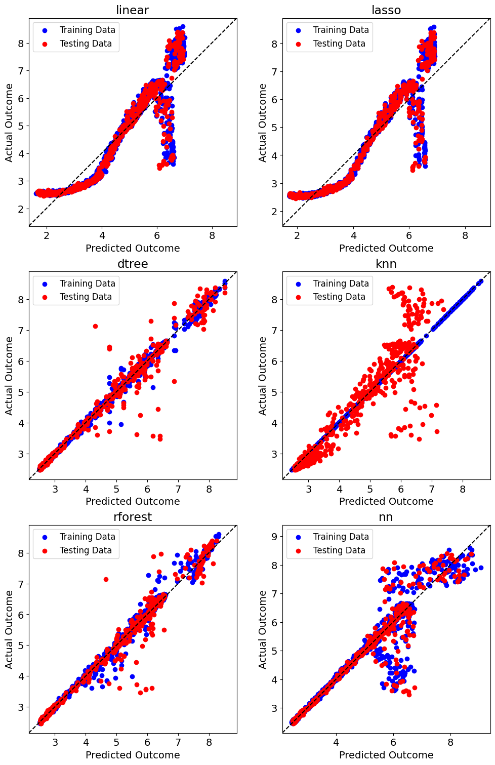
The performance differences between rforest/dtree with the other models is apparent along with the overfitting of knn. The predictions of rforest and dtree are closely spread along \(y=x\) while the knn test predictions are over-predicted.

Similarly, the validation_plot function produces validation plots that show the absolute relative error for each prediction.

fig, axarr = plt.subplots(models.shape[0], models.shape[1], figsize=(17,22))

y = ["Max4Pin"]

for i in range(models.shape[0]):
    for j in range(models.shape[1]):
        plt.sca(axarr[i, j])
        axarr[i, j] = postprocessor.validation_plot(model_type=models[i, j], y=y)
        axarr[i, j].set_title(models[i, j])

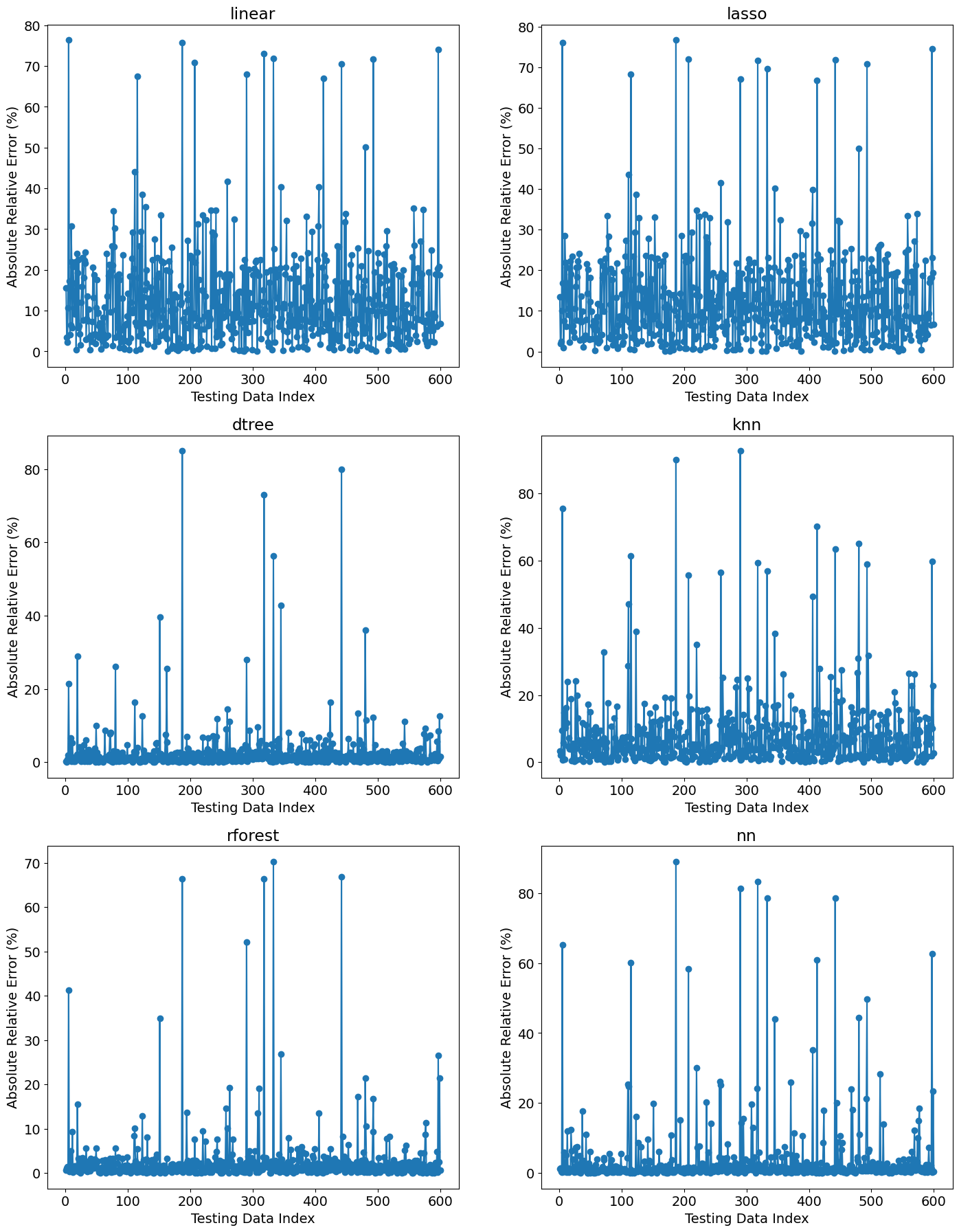
The performance of the models is best represented by the magnitudes observed on the y-axis; however, even rforest and dtree get as high as \(>3.0\%\) error.

Finally, the learning curve of the most performant nn is shown by nn_learning_plot.

fig, ax = plt.subplots(figsize=(8,8))
ax = postprocessor.nn_learning_plot()

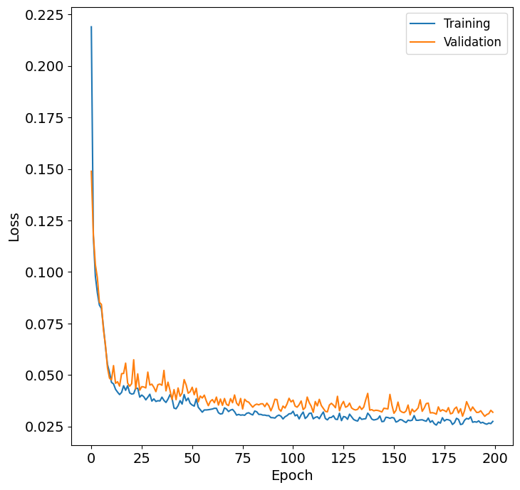
The neural network learning curve above shows that there is no overfitting as traning and validation are very similiar. The converges to 0.025 which is an acceptable number.

References

1. 13. 1. Radaideh, B. Forget, and K. Shirvan, “Large-scale design optimisation of boiling water re- actor bundles with neuroevolution,” Annals of Nuclear Energy, vol. 160, p. 108355, 2021.