NEACRP C1 Rod Ejection Accident

Inputs

• rod_worth: Reactivity worth of the ejected rod

• beta: Delayed neutron fraction

• h_gap: Gap conductance (\(\frac{W}{m^2 \cdot K}\))

• gamma_frac: Direct heating fraction

Outputs

• max_power: peak power (\(\% FP\))

• burst_width: Width of power burst (\(s\))

• max_TF: Max fuel centerline temperature (\(K\))

• avg_Tcool: Average coolant temperature at the outlet (\(K\))

The NEACRP C1 rod ejection accident (REA) data represents one benchmark for reactor transient analysis. The data set is used to find the relationship between the REA/reactor parameters and the power/thermal behavior of the system during/after the event. Therefore, the data set is constructed by perturbing the inputs listed above—the corresponding output results in values of interest to the safety analysis of the transient. The data were generated using deterministic simulations by the PARCS code, where the data set size includes 2000 samples. The goal is to use pyMAISE to build, tune, and compare the performance of various ML models in predicting the transient outcomes based on the REA properties.

from pyMAISE.datasets import load_rea
from pyMAISE.preprocessing import correlation_matrix, train_test_split, scale_data
import pyMAISE as mai

import time
import numpy as np
import matplotlib.pyplot as plt
from scipy.stats import uniform, randint
from sklearn.preprocessing import MinMaxScaler

# Plot settings
matplotlib_settings = {
    "font.size": 12,
    "legend.fontsize": 11,
    "figure.figsize": (8, 8)
}
plt.rcParams.update(**matplotlib_settings)

Preprocessing

We define a pyMAISE regression problem and load the REA data.

global_settings = mai.init(
    problem_type=mai.ProblemType.REGRESSION,   # Define a regression problem
    cuda_visible_devices="-1"                  # Use CPU only
)
data, inputs, outputs = load_rea()

As stated the data set consists of 4 inputs:

inputs

<xarray.DataArray (index: 2000, variable: 4)>
array([[8.63781014e-03, 7.57558927e-03, 1.37279819e+04, 2.39566042e-02],
       [9.25495922e-03, 7.52915145e-03, 9.37021808e+03, 1.97072356e-02],
       [8.04631321e-03, 7.64737606e-03, 9.96254385e+03, 2.00446440e-02],
       ...,
       [8.72425595e-03, 7.47087165e-03, 1.10723962e+04, 1.53597012e-02],
       [9.11742702e-03, 7.49571772e-03, 1.08772638e+04, 1.73452589e-02],
       [8.35065112e-03, 7.63110349e-03, 1.34164011e+04, 1.71329041e-02]])
Coordinates:
  * index     (index) int64 0 1 2 3 4 5 6 ... 1993 1994 1995 1996 1997 1998 1999
  * variable  (variable) object 'rod_worth' 'beta' 'h_gap' 'gamma_frac'

xarray.DataArray

• index: 2000
• variable: 4

• 0.008638 0.007576 1.373e+04 0.02396 ... 0.007631 1.342e+04 0.01713

  array([[8.63781014e-03, 7.57558927e-03, 1.37279819e+04, 2.39566042e-02],
         [9.25495922e-03, 7.52915145e-03, 9.37021808e+03, 1.97072356e-02],
         [8.04631321e-03, 7.64737606e-03, 9.96254385e+03, 2.00446440e-02],
         ...,
         [8.72425595e-03, 7.47087165e-03, 1.10723962e+04, 1.53597012e-02],
         [9.11742702e-03, 7.49571772e-03, 1.08772638e+04, 1.73452589e-02],
         [8.35065112e-03, 7.63110349e-03, 1.34164011e+04, 1.71329041e-02]])

• Coordinates: (2)
  • index
    (index)
    int64
    0 1 2 3 4 ... 1996 1997 1998 1999

    array([   0,    1,    2, ..., 1997, 1998, 1999])

  • variable
    (variable)
    object
    'rod_worth' 'beta' ... 'gamma_frac'

    array(['rod_worth', 'beta', 'h_gap', 'gamma_frac'], dtype=object)

• Indexes: (2)
  • index
    PandasIndex

    PandasIndex(RangeIndex(start=0, stop=2000, step=1, name='index'))

  • variable
    PandasIndex

    PandasIndex(Index(['rod_worth', 'beta', 'h_gap', 'gamma_frac'], dtype='object', name='variable'))

• Attributes: (0)

and 4 outputs with 2000 total data points:

outputs

<xarray.DataArray (index: 2000, variable: 4)>
array([[1.81210000e+02, 3.15000000e-01, 9.18300000e+02, 5.61119081e+02],
       [4.74590000e+02, 2.50000000e-01, 9.65200000e+02, 5.62030035e+02],
       [4.40830000e+01, 4.25000000e-01, 8.75700000e+02, 5.60194700e+02],
       ...,
       [2.55980000e+02, 2.90000000e-01, 9.36100000e+02, 5.61324028e+02],
       [4.27900000e+02, 2.55000000e-01, 9.57800000e+02, 5.61933922e+02],
       [9.69710000e+01, 3.80000000e-01, 8.98000000e+02, 5.60613781e+02]])
Coordinates:
  * index     (index) int64 0 1 2 3 4 5 6 ... 1993 1994 1995 1996 1997 1998 1999
  * variable  (variable) object 'max_power' 'burst_width' 'max_Tf' 'avg_Tcool'

xarray.DataArray

• index: 2000
• variable: 4

• 181.2 0.315 918.3 561.1 474.6 0.25 ... 561.9 96.97 0.38 898.0 560.6

  array([[1.81210000e+02, 3.15000000e-01, 9.18300000e+02, 5.61119081e+02],
         [4.74590000e+02, 2.50000000e-01, 9.65200000e+02, 5.62030035e+02],
         [4.40830000e+01, 4.25000000e-01, 8.75700000e+02, 5.60194700e+02],
         ...,
         [2.55980000e+02, 2.90000000e-01, 9.36100000e+02, 5.61324028e+02],
         [4.27900000e+02, 2.55000000e-01, 9.57800000e+02, 5.61933922e+02],
         [9.69710000e+01, 3.80000000e-01, 8.98000000e+02, 5.60613781e+02]])

• Coordinates: (2)
  • index
    (index)
    int64
    0 1 2 3 4 ... 1996 1997 1998 1999

    array([   0,    1,    2, ..., 1997, 1998, 1999])

  • variable
    (variable)
    object
    'max_power' ... 'avg_Tcool'

    array(['max_power', 'burst_width', 'max_Tf', 'avg_Tcool'], dtype=object)

• Indexes: (2)
  • index
    PandasIndex

    PandasIndex(RangeIndex(start=0, stop=2000, step=1, name='index'))

  • variable
    PandasIndex

    PandasIndex(Index(['max_power', 'burst_width', 'max_Tf', 'avg_Tcool'], dtype='object', name='variable'))

• Attributes: (0)

Prior to constructing any models we can get a surface understanding of the data set with a correlation matrix.

correlation_matrix(data)
plt.show()

A positive correlation exists between average coolant temperature and max fuel temperature, max power, and rod worth. The delayed neutron fraction and burst width negatively correlate with max fuel temperature, max power, and rod worth.

We train/test split into 70%/30% and scale inputs and outputs using min-max scaling to optimize model training.

xtrain, xtest, ytrain, ytest = train_test_split(data=[inputs, outputs], test_size=0.3)
xtrain, xtest, xscaler = scale_data(xtrain, xtest, scaler=MinMaxScaler())
ytrain, ytest, yscaler = scale_data(ytrain, ytest, scaler=MinMaxScaler())

Model Initialization

We will examine the performance of 6 regression models in this data set:

• linear: Linear,

• lasso: Lasso,

• decision tree: DT,

• random forest: RF,

• k-nearest neighbors regression: KN,

• dense feedforward neural network: FNN.

For hyperparameter tuning, we initialize all classical models as scikit-learn defaults. For the FNN, we define input and output layers with possible dropout layers. These layers include hyperparameter tuning of their number of nodes, the use of sublayers, and the dropout rate. The dense hidden layers include tuning of their depth.

model_settings = {
    "models": ["Linear", "Lasso", "DT", "RF", "KN", "FNN"],
    "FNN": {
        "structural_params": {
            "Dense_hidden": {
                "num_layers": mai.Int(min_value=0, max_value=3),
                "units": mai.Int(min_value=25, max_value=400),
                "activation": "relu",
                "kernel_initializer": "normal",
                "sublayer": mai.Choice(["Dropout_hidden", "None"]),
                "Dropout_hidden": {
                    "rate": mai.Float(min_value=0.4, max_value=0.6),
                },
            },
            "Dense_output": {
                "units": ytrain.shape[-1],
                "activation": "linear",
                "kernel_initializer": "normal",
            },
        },
        "optimizer": "Adam",
        "Adam": {
            "learning_rate": mai.Float(min_value=1e-5, max_value=0.001),
        },
        "compile_params": {
            "loss": "mean_absolute_error",
            "metrics": ["mean_absolute_error"],
        },
        "fitting_params": {
            "batch_size": mai.Choice([8, 16, 32]),
            "epochs": 50,
            "validation_split": 0.15,
        },
    },
}
tuner = mai.Tuner(xtrain, ytrain, model_settings=model_settings)

Hyperparameter Tuning

We use a random search with 200 iterations and five cross-validation splits (1000 fits per model) for the classical models. The hyperparameter search space is defined for all but linear regression in which the default scikit-learn configuration will be tested. For the FNN, we use a Bayesian search with 50 iterations and five cross-validation splits (250 fits total). This offers possible convergence on an optimal configuration without taking excessive time. Classical models tend to be simpler than neural networks, so many random search iterations are possible.

random_search_spaces = {
    "Lasso": {
        "alpha": uniform(loc=0.0001, scale=0.0099), # 0.0001 - 0.01
    },
    "DT": {
        "max_depth": randint(low=5, high=50), # 5 - 50
        "max_features": [None, "sqrt", "log2", 2, 4, 6],
        "min_samples_split": randint(low=2, high=20), # 2 - 20
        "min_samples_leaf": randint(low=1, high=20), # 1 - 20
    },
    "RF": {
        "n_estimators": randint(low=50, high=200), # 50 - 200
        "criterion": ["squared_error", "absolute_error", "poisson"],
        "min_samples_split": randint(low=2, high=20), # 2 - 20
        "min_samples_leaf": randint(low=1, high=20), # 1 - 20
        "max_features": [None, "sqrt", "log2", 2, 4, 6],
    },
    "KN": {
        "n_neighbors": randint(low=1, high=20), # 1 - 20
        "weights": ["uniform", "distance"],
        "leaf_size": randint(low=1, high=30), # 1 - 30
        "p": randint(low=1, high=10), # 1 - 10
    },
}
start = time.time()
random_search_configs = tuner.random_search(
    param_spaces=random_search_spaces,
    n_iter=200,
    n_jobs=6,
    cv=5,
)
bayesian_search_configs = tuner.nn_bayesian_search(
    objective="r2_score",
    max_trials=50,
    cv=5,
)
print("Hyperparameter tuning took " + str((time.time() - start) / 60) + " minutes to process.")

Hyperparameter tuning took 43.74738088051478 minutes to process.

Here is the convergence plot of the Bayesian search:

ax = tuner.convergence_plot(model_types="FNN")
ax.set_ylim([0, 1])
plt.show()

Post-processing

We can now pass these parameter configurations to the pyMAISE.PostProcessor for model evaluation. We increase the neural network epochs to 200 to improve their fit.

postprocessor = mai.PostProcessor(
    data=(xtrain, xtest, ytrain, ytest),
    model_configs=[random_search_configs, bayesian_search_configs],
    new_model_settings={
        "FNN": {"fitting_params": {"epochs": 200}},
    },
    yscaler=yscaler,
)

To compare the performance of these models, we compute five metrics for both the training and testing data:

• mean absolute percentage error: MAPE \(=\frac{100}{n} \sum_{i = 1}^n \frac{|y_i - \hat{y}_i|}{\text{max}(\epsilon, |y_i|)}\),

• root mean squared error RMSE \(=\sqrt{\frac{1}{n}\sum^n_{i = 1}(y_i - \hat{y}_i)^2}\),

• root mean squared percentage error RMSPE \(= \sqrt{\frac{1}{n}\sum_{i = 1}^n\Big(\frac{y_i - \hat{y}_i}{\text{max}(\epsilon, |y_i|)}\Big)^2}\),

• mean absolute error MAE = \(=\frac{1}{n}\sum^n_{i = 1}|y_i - \hat{y}_i|\),

• and r-squared R2 \(=1 - \frac{\sum^n_{i = 1}(y_i - \hat{y}_i)^2}{\sum^n_{i = 1}(y_i - \bar{y}_i)^2}\),

where \(y\) is the actual outcome, \(\bar{y}\) is the average outcome, \(\hat{y}\) is the model predicted outcome, and \(n\) is the number of observations. The averaged performance metrics are shown below.

postprocessor.metrics(y="max_power").drop("Parameter Configurations", axis=1)

	Model Types	Train R2	Train MAE	Train MAPE	Train RMSE	Train RMSPE	Test R2	Test MAE	Test MAPE	Test RMSE	Test RMSPE
24	FNN	0.999852	1.699854	1.256283	2.468033	4.722631	0.999826	1.835816	1.458129	2.916537	5.567953
21	FNN	0.999918	1.127129	0.796116	1.833239	1.552226	0.999801	1.365720	0.861927	3.126094	1.616800
25	FNN	0.999672	3.138061	2.933183	3.676620	4.800341	0.999609	3.292828	3.106852	4.377233	5.097466
22	FNN	0.999237	4.904743	3.195386	5.608668	4.712873	0.999250	5.007710	3.405431	6.061238	5.493813
23	FNN	0.998411	5.961130	2.895374	8.091014	5.092613	0.998364	6.257894	3.002727	8.952768	5.261215
11	RF	0.996629	5.304325	2.319889	11.785955	3.832069	0.991116	11.428480	4.791165	20.865264	6.736489
12	RF	0.996067	5.766477	2.480829	12.729718	4.087183	0.990400	11.645784	4.777181	21.690159	6.706852
14	RF	0.994627	7.015301	3.009012	14.880166	4.906394	0.989131	12.360400	5.004573	23.079143	6.963417
13	RF	0.995233	6.186133	2.708629	14.015775	4.417449	0.988940	11.386044	4.662103	23.281506	6.891529
15	RF	0.994476	6.441467	2.785306	15.086559	4.779654	0.988741	11.919416	4.847624	23.490204	6.882004
8	DT	0.994044	9.081504	4.054642	15.665554	5.648996	0.979416	19.844302	8.433758	31.761324	11.637799
7	DT	0.991804	11.160518	4.976151	18.377108	6.808786	0.978735	20.352947	8.773481	32.281932	11.976627
9	DT	0.996262	6.352290	2.833096	12.410041	4.119718	0.978387	19.657342	8.480095	32.545247	12.095232
6	DT	0.995151	8.098864	3.634065	14.135962	5.247021	0.977442	19.895052	8.472278	33.249146	12.096130
10	DT	0.991569	11.149304	4.940116	18.639007	7.087156	0.976981	20.664656	9.041800	33.587340	12.532541
17	KN	1.000000	0.000000	0.000000	0.000000	0.000000	0.969696	22.108553	10.746691	38.537273	16.923626
19	KN	0.982434	16.356414	8.072365	26.904226	11.911547	0.966066	24.738338	11.858489	40.779695	18.464650
20	KN	0.982434	16.356414	8.072365	26.904226	11.911547	0.966066	24.738338	11.858489	40.779695	18.464650
16	KN	1.000000	0.000000	0.000000	0.000000	0.000000	0.964889	23.790712	11.232340	41.481149	17.192940
18	KN	1.000000	0.000000	0.000000	0.000000	0.000000	0.963346	23.195838	11.111103	42.382962	17.617189
0	Linear	0.885868	49.233342	66.142991	68.577987	234.878112	0.872378	54.203537	80.827036	79.084691	290.808312
1	Lasso	0.885596	49.217072	64.566529	68.659435	228.969793	0.871874	54.150838	78.816899	79.240490	283.345055
2	Lasso	0.885506	49.222476	64.328463	68.686572	228.061933	0.871749	54.152451	78.516695	79.279058	282.196401
3	Lasso	0.885442	49.228422	64.180094	68.705780	227.487558	0.871664	54.155169	78.327780	79.305498	281.469416
4	Lasso	0.884287	49.352720	62.376050	69.051257	220.317005	0.870263	54.208453	75.965568	79.737266	272.380821
5	Lasso	0.884053	49.385849	62.059549	69.121055	218.994281	0.869993	54.226020	75.531912	79.820175	270.704688

For max power, all but linear and lasso regression have tested \(R^2\) greater than 0.95. The FNN and random forest models performed exceptionally with test \(R^2\) greater than 0.99.

postprocessor.metrics(y="burst_width").drop("Parameter Configurations", axis=1)

	Model Types	Train R2	Train MAE	Train MAPE	Train RMSE	Train RMSPE	Test R2	Test MAE	Test MAPE	Test RMSE	Test RMSPE
25	FNN	0.993917	0.004330	1.108645	0.009463	1.745603	0.989397	0.005266	1.325654	0.014530	3.550121
24	FNN	0.995823	0.003956	1.080418	0.007841	1.715023	0.989178	0.004937	1.273542	0.014679	3.780443
21	FNN	0.993285	0.006719	2.169849	0.009942	2.688709	0.985970	0.007982	2.412915	0.016714	4.452748
22	FNN	0.993884	0.004217	1.124124	0.009488	1.816849	0.983470	0.005470	1.344439	0.018142	4.199390
11	RF	0.979174	0.004123	0.984087	0.017509	1.810321	0.970323	0.007950	1.806846	0.024309	3.983300
15	RF	0.966754	0.005200	1.202897	0.022121	2.366208	0.968834	0.008271	1.839297	0.024911	3.941832
23	FNN	0.968362	0.007532	1.726643	0.021580	3.430110	0.964017	0.009178	1.996662	0.026767	4.399339
14	RF	0.973912	0.005283	1.262896	0.019596	2.363813	0.964002	0.008324	1.839627	0.026773	3.955729
12	RF	0.978590	0.004373	1.051177	0.017752	1.959277	0.963183	0.008101	1.821587	0.027076	4.222441
13	RF	0.980769	0.004929	1.183498	0.016825	2.269449	0.959128	0.008283	1.814489	0.028528	4.034780
6	DT	0.984433	0.005017	1.291388	0.015137	2.004014	0.958171	0.011373	2.740013	0.028860	4.374540
9	DT	0.985966	0.004210	1.064954	0.014372	1.757386	0.958043	0.011360	2.734582	0.028904	4.376369
8	DT	0.980703	0.005628	1.399546	0.016854	2.231994	0.929063	0.012128	2.787213	0.037583	4.629539
7	DT	0.978080	0.006520	1.636774	0.017963	2.539207	0.927618	0.012259	2.800895	0.037964	4.671377
10	DT	0.968644	0.007128	1.735428	0.021484	3.175024	0.925357	0.012628	2.884700	0.038552	5.013745
19	KN	0.926553	0.009842	2.270713	0.032880	3.895120	0.858403	0.016922	3.688973	0.053098	7.461661
20	KN	0.926553	0.009842	2.270713	0.032880	3.895120	0.858403	0.016922	3.688973	0.053098	7.461661
16	KN	1.000000	0.000000	0.000000	0.000000	0.000000	0.855540	0.016597	3.556377	0.053633	7.155635
17	KN	1.000000	0.000000	0.000000	0.000000	0.000000	0.840776	0.017002	3.536212	0.056306	7.438459
18	KN	1.000000	0.000000	0.000000	0.000000	0.000000	0.830735	0.016653	3.462633	0.058055	7.046017
0	Linear	0.573610	0.033512	9.124697	0.079223	12.597111	0.552214	0.040083	10.298337	0.094426	14.781481
1	Lasso	0.573004	0.032137	8.612343	0.079279	11.972884	0.549173	0.038690	9.750295	0.094746	14.137907
2	Lasso	0.572826	0.031939	8.537622	0.079295	11.879015	0.548654	0.038477	9.666154	0.094800	14.039045
3	Lasso	0.572701	0.031814	8.490732	0.079307	11.820095	0.548315	0.038342	9.613070	0.094836	13.976949
4	Lasso	0.570241	0.030325	7.926108	0.079535	11.117745	0.543321	0.036740	8.976951	0.095359	13.233395
5	Lasso	0.569601	0.030061	7.825759	0.079594	10.995593	0.542241	0.036462	8.865812	0.095471	13.103219

For burst width k-nearest neighbors, decision tree, lasso, and linear regression largely struggled. K-nearest neighbors are overfit. The top performers were the FNN and random forest models; however, the FNN was more consistent between training and testing.

postprocessor.metrics(y="max_Tf").drop("Parameter Configurations", axis=1)

	Model Types	Train R2	Train MAE	Train MAPE	Train RMSE	Train RMSPE	Test R2	Test MAE	Test MAPE	Test RMSE	Test RMSPE
25	FNN	0.999532	0.545938	0.059499	0.754793	0.082855	0.999426	0.606922	0.066115	0.896838	0.099307
24	FNN	0.999385	0.644342	0.070049	0.865333	0.096562	0.999283	0.680491	0.074382	1.001813	0.114124
21	FNN	0.999292	0.739538	0.080567	0.928501	0.103014	0.999018	0.827692	0.090418	1.172481	0.131682
22	FNN	0.998933	0.985210	0.106235	1.139831	0.122799	0.998745	1.058086	0.114233	1.325851	0.144121
23	FNN	0.998107	0.963719	0.106022	1.518266	0.174202	0.997697	1.064322	0.117188	1.796139	0.204868
11	RF	0.994683	1.523018	0.164220	2.544729	0.275500	0.988703	2.763608	0.298509	3.977785	0.429070
12	RF	0.993695	1.696249	0.182596	2.771042	0.298416	0.987736	2.843847	0.307049	4.144432	0.448508
15	RF	0.991260	1.993675	0.214964	3.262472	0.353055	0.985931	3.004872	0.324483	4.438993	0.476232
14	RF	0.990509	2.240935	0.241357	3.399858	0.366108	0.985137	3.188399	0.344184	4.562532	0.493237
13	RF	0.990368	2.295046	0.247355	3.425057	0.366766	0.983783	3.247793	0.350634	4.765852	0.513841
0	Linear	0.984854	2.629205	0.286122	4.294806	0.489630	0.981907	3.026196	0.330220	5.033933	0.575311
1	Lasso	0.984410	2.552006	0.278191	4.357388	0.499009	0.980912	2.969868	0.324696	5.170536	0.592588
2	Lasso	0.984261	2.550351	0.278073	4.378057	0.501578	0.980687	2.970023	0.324810	5.200957	0.596208
3	Lasso	0.984156	2.549879	0.278061	4.392633	0.503356	0.980534	2.971079	0.324990	5.221468	0.598627
4	Lasso	0.982099	2.651108	0.289520	4.669081	0.535140	0.977952	3.086539	0.338240	5.556995	0.636938
5	Lasso	0.981565	2.692435	0.294083	4.738293	0.542853	0.977335	3.132921	0.343409	5.634228	0.645574
9	DT	0.993595	1.842810	0.198248	2.792917	0.299221	0.975033	4.437028	0.479015	5.913407	0.639559
6	DT	0.990878	2.345429	0.252307	3.333039	0.357373	0.974013	4.584203	0.494902	6.032961	0.652280
8	DT	0.989335	2.553981	0.274939	3.603947	0.386728	0.973060	4.547281	0.491762	6.142587	0.672752
7	DT	0.986161	3.030964	0.326486	4.105373	0.441465	0.971338	4.701304	0.508913	6.335875	0.693934
17	KN	1.000000	0.000000	0.000000	0.000000	0.000000	0.971213	3.884504	0.423387	6.349685	0.706129
10	DT	0.984997	3.143687	0.338816	4.274556	0.461723	0.969568	4.896121	0.529683	6.528658	0.712333
16	KN	1.000000	0.000000	0.000000	0.000000	0.000000	0.969379	4.097332	0.445330	6.548905	0.722502
19	KN	0.984872	2.899286	0.315172	4.292222	0.474244	0.968884	4.363556	0.474343	6.601565	0.730224
20	KN	0.984872	2.899286	0.315172	4.292222	0.474244	0.968884	4.363556	0.474343	6.601565	0.730224
18	KN	1.000000	0.000000	0.000000	0.000000	0.000000	0.967451	3.969212	0.431782	6.751909	0.748772

Max fuel temperature is a more linear label, with all models performing well with \(R^2\) greater than 0.95. Once again, the FNN and random forest models were the top-performing models.

postprocessor.metrics(y="avg_Tcool").drop("Parameter Configurations", axis=1)

	Model Types	Train R2	Train MAE	Train MAPE	Train RMSE	Train RMSPE	Test R2	Test MAE	Test MAPE	Test RMSE	Test RMSPE
24	FNN	0.999877	0.006093	0.001085	0.008180	0.001456	0.999890	0.005894	0.001050	0.008247	0.001468
25	FNN	0.999911	0.004936	0.000879	0.006966	0.001240	0.999878	0.005646	0.001006	0.008693	0.001547
21	FNN	0.999715	0.011354	0.002024	0.012467	0.002223	0.999724	0.011706	0.002087	0.013044	0.002325
23	FNN	0.999554	0.012537	0.002234	0.015601	0.002778	0.999495	0.013301	0.002370	0.017658	0.003142
22	FNN	0.998758	0.024142	0.004301	0.026039	0.004637	0.998844	0.024489	0.004363	0.026710	0.004756
11	RF	0.996797	0.025205	0.004489	0.041825	0.007442	0.990428	0.051421	0.009158	0.076863	0.013681
12	RF	0.996255	0.027642	0.004923	0.045223	0.008047	0.990037	0.052449	0.009341	0.078417	0.013957
15	RF	0.994865	0.031991	0.005698	0.052956	0.009424	0.988644	0.054895	0.009776	0.083719	0.014900
14	RF	0.994204	0.035662	0.006352	0.056263	0.010012	0.987811	0.058346	0.010391	0.086737	0.015438
13	RF	0.994462	0.035716	0.006361	0.054994	0.009787	0.986936	0.059233	0.010549	0.089797	0.015982
0	Linear	0.982404	0.069074	0.012309	0.098028	0.017469	0.981088	0.075828	0.013512	0.108039	0.019252
17	KN	1.000000	0.000000	0.000000	0.000000	0.000000	0.980886	0.076744	0.013671	0.108616	0.019339
1	Lasso	0.982246	0.070077	0.012487	0.098466	0.017542	0.980840	0.076791	0.013682	0.108745	0.019373
2	Lasso	0.982196	0.070258	0.012519	0.098604	0.017566	0.980773	0.076979	0.013715	0.108935	0.019406
3	Lasso	0.982161	0.070374	0.012539	0.098701	0.017583	0.980727	0.077111	0.013738	0.109066	0.019429
4	Lasso	0.981472	0.072159	0.012856	0.100590	0.017914	0.979899	0.079219	0.014112	0.111384	0.019836
5	Lasso	0.981293	0.072571	0.012929	0.101075	0.017999	0.979694	0.079717	0.014201	0.111950	0.019935
18	KN	1.000000	0.000000	0.000000	0.000000	0.000000	0.979269	0.079611	0.014180	0.113116	0.020136
8	DT	0.994103	0.039421	0.007022	0.056748	0.010102	0.979068	0.083381	0.014852	0.113664	0.020238
16	KN	1.000000	0.000000	0.000000	0.000000	0.000000	0.978906	0.081871	0.014583	0.114102	0.020314
9	DT	0.996396	0.029075	0.005179	0.044366	0.007896	0.978672	0.084051	0.014972	0.114733	0.020430
6	DT	0.994959	0.036084	0.006428	0.052467	0.009340	0.978621	0.083848	0.014935	0.114871	0.020454
19	KN	0.988262	0.058839	0.010482	0.080064	0.014257	0.977642	0.086407	0.015392	0.117471	0.020918
20	KN	0.988262	0.058839	0.010482	0.080064	0.014257	0.977642	0.086407	0.015392	0.117471	0.020918
7	DT	0.992006	0.047951	0.008542	0.066071	0.011764	0.977490	0.088286	0.015726	0.117869	0.020987
10	DT	0.991517	0.048225	0.008591	0.068062	0.012117	0.974911	0.090845	0.016181	0.124440	0.022155

Average coolant temperature was also well predicted by all models.

postprocessor.metrics().drop(
    ["Parameter Configurations", "Train MAE", "Test MAE", "Train RMSE", "Test RMSE"],
    axis=1,
)

	Model Types	Train R2	Train MAPE	Train RMSPE	Test R2	Test MAPE	Test RMSPE
25	FNN	0.998258	1.025552	1.657510	0.997077	1.124907	2.187110
24	FNN	0.998735	0.601959	1.633918	0.997045	0.701776	2.365997
21	FNN	0.998053	0.762139	1.086543	0.996128	0.841837	1.550889
22	FNN	0.997703	1.107512	1.664289	0.995077	1.217116	2.460520
23	FNN	0.991109	1.182568	2.174926	0.989893	1.279736	2.467141
11	RF	0.991821	0.868171	1.481333	0.985142	1.726420	2.790635
15	RF	0.986839	1.052216	1.877085	0.983037	1.755295	2.828742
12	RF	0.991152	0.929881	1.588231	0.982839	1.728789	2.847940
14	RF	0.988313	1.129904	1.911582	0.981520	1.799693	2.856955
13	RF	0.990208	1.036461	1.765863	0.979697	1.709444	2.864033
9	DT	0.993055	1.025369	1.546055	0.972534	2.927166	4.282898
6	DT	0.991355	1.296047	1.904437	0.972062	2.930532	4.285851
8	DT	0.989546	1.434037	2.069455	0.965152	2.931896	4.240082
7	DT	0.987013	1.736988	2.450306	0.963796	3.024754	4.340731
10	DT	0.984182	1.755738	2.684005	0.961704	3.118091	4.570194
19	KN	0.970530	2.667183	4.073792	0.942749	4.009299	6.669363
20	KN	0.970530	2.667183	4.073792	0.942749	4.009299	6.669363
16	KN	1.000000	0.000000	0.000000	0.942178	3.812157	6.272848
17	KN	1.000000	0.000000	0.000000	0.940643	3.679990	6.271888
18	KN	1.000000	0.000000	0.000000	0.935200	3.754925	6.358028
0	Linear	0.856684	18.891530	61.995581	0.846897	22.867276	76.546089
1	Lasso	0.856314	18.367387	60.364807	0.845700	22.226393	74.523731
2	Lasso	0.856198	18.289169	60.115023	0.845466	22.130344	74.212765
3	Lasso	0.856115	18.240356	59.957148	0.845310	22.069895	74.016105
4	Lasso	0.854525	17.651134	57.996951	0.842859	21.323718	71.567748
5	Lasso	0.854128	17.548080	57.637682	0.842316	21.188834	71.118354

Overall, the top-performing models are the FNNs, some of which are above 0.99 \(R^2\) for training and testing data sets. Linear and lasso regression were the worst-performing models.

Below are the hyperparameter configurations of each of the top-performing models.

for model in ["Lasso", "DT", "RF", "KN", "FNN"]:
    postprocessor.print_model(model_type=model)
    print()

Model Type: Lasso
  alpha: 0.00020315144347484598

Model Type: DT
  max_depth: 26
  max_features: None
  min_samples_leaf: 2
  min_samples_split: 4

Model Type: RF
  criterion: squared_error
  max_features: None
  min_samples_leaf: 2
  min_samples_split: 2
  n_estimators: 112

Model Type: KN
  leaf_size: 26
  n_neighbors: 3
  p: 2
  weights: uniform

Model Type: FNN
  Structural Hyperparameters
    Layer: Dense_hidden_0
      units: 326
      sublayer: None
    Layer: Dense_hidden_1
      units: 127
      sublayer: None
    Layer: Dense_output_0
  Compile/Fitting Hyperparameters
    Adam_learning_rate: 0.0009444837105276597
    batch_size: 8
Model: "FNN"
_________________________________________________________________
 Layer (type)                Output Shape              Param #
=================================================================
 Dense_hidden_0 (Dense)      (None, 326)               1630

 Dense_hidden_1 (Dense)      (None, 127)               41529

 Dense_output_0 (Dense)      (None, 4)                 512

=================================================================
Total params: 43671 (170.59 KB)
Trainable params: 43671 (170.59 KB)
Non-trainable params: 0 (0.00 Byte)
_________________________________________________________________

Below is the network plot for the FNN.

postprocessor.nn_network_plot(
    to_file="./supporting/rod_ejection_network.png",
    show_shapes=True,
    show_layer_names=True,
    expand_nested=True,
    show_layer_activations=True,
)

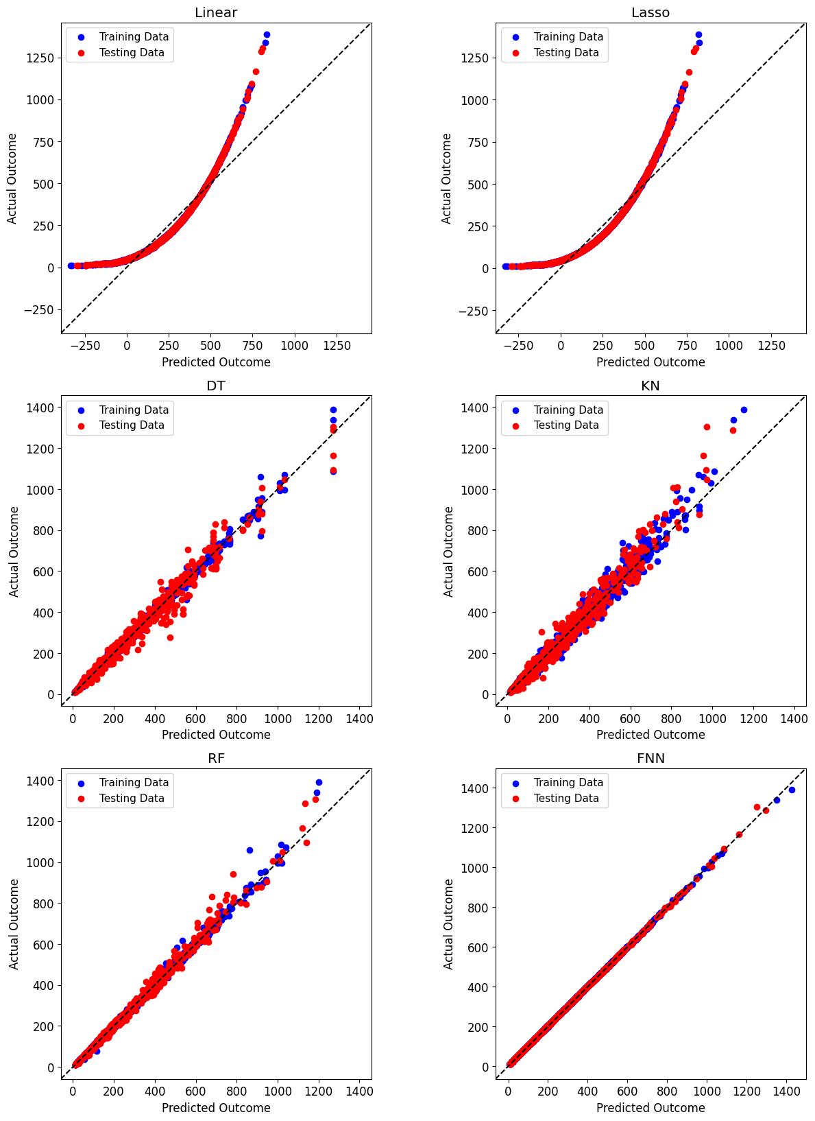
We can visualize the performance of each model with diagonal validation plots. These plots show the predicted output to the actual production. The performance of FNN is apparent with the spread close around \(y= x\). Random forest, k-nearest neighbors, and decision tree performed relatively well on all outputs. Burst width is the most difficult to predict for all the models.

def performance_plot(meth, output):
    models = np.array([["Linear", "Lasso"], ["DT", "KN"], ["RF", "FNN"]])
    fig, axarr = plt.subplots(models.shape[0], models.shape[1], figsize=(15,20))
    for i in range(models.shape[0]):
        for j in range(models.shape[1]):
            plt.sca(axarr[i, j])
            axarr[i, j] = meth(model_type=models[i, j], y=[output])
            axarr[i, j].set_title(models[i, j])


performance_plot(postprocessor.diagonal_validation_plot, "max_power")
plt.show()

performance_plot(postprocessor.diagonal_validation_plot, "burst_width")
plt.show()

performance_plot(postprocessor.diagonal_validation_plot, "max_Tf")
plt.show()

performance_plot(postprocessor.diagonal_validation_plot, "avg_Tcool")
plt.show()

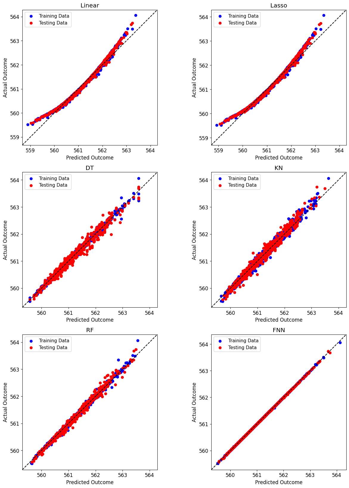
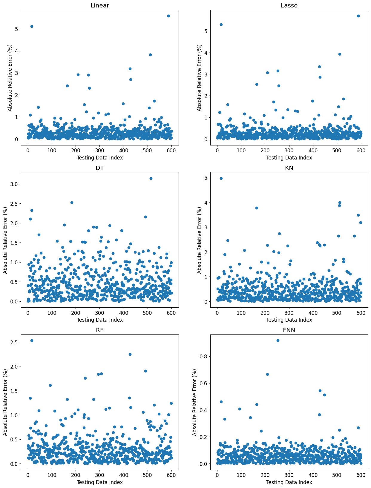
The validation plots for all outputs are given below. Based on the scaling of the \(y\)-axis, we can see that the FNNs performed the best. Both the diagonal validation and validation plots agree with the performance metrics presented above.

performance_plot(postprocessor.validation_plot, "max_power")
plt.show()

performance_plot(postprocessor.validation_plot, "burst_width")
plt.show()

performance_plot(postprocessor.validation_plot, "max_Tf")
plt.show()

performance_plot(postprocessor.validation_plot, "avg_Tcool")
plt.show()

Finally, the most learning curve for the most performant FNN is shown below. It shows no overfitting, as the validation curve follows the training curve closely.

postprocessor.nn_learning_plot()
plt.show()