Binary Anomaly Detection

Inputs

The 14 waveform inputs are:

A+IGBT-I: current: Current passing through the IGBT switch of phase A+ in Qa1 (\(A\))
A+*IGBT-I: current: Current passing through the IGBT switch of phase A+* in Qa3 (\(A\))
B+IGBT-I: current: Current passing through the IGBT switch of phase B+ in Qb1 (\(A\))
B+*IGBT-I: current: Current passing through the IGBT switch of phase B+* in Qb3 (\(A\))
C+IGBT-I: current: Current passing through the IGBT switch of phase C+ in Qc1 (\(A\))
C+*IGBT-I: current: Current passing through the IGBT switch of phase C+* in Qc3 (\(A\))
A-Flux: Magnetic flux density for phase A in transformer XA (\(-\))
B-Flux: Magnetic flux density for phase B in transformer XB (\(-\))
C-Flux: Magnetic flux density for phase C in transformer XC (\(-\))
Mod-V: Modulator voltage (\(V\))
Mod-I: Modulator current (\(A\))
CB-I: Cap bank current (\(-\))
CB-V: Cap bank voltage (\(V\))
DV/DT: Time derivative change of the Mod-V voltage (\(-\))

Output

Class_Run/Class_Fault: Whether a waveform is a part of a system fault

This benchmark analyzes a measured dataset originating from [RPW+22, RPW+23] for the high voltage converter modulators (HVCM) of the Spallation Neutron Source facility. While this data does not originate from a nuclear power plant, its nature is similar to that found from measured sensor data in nuclear power plants.

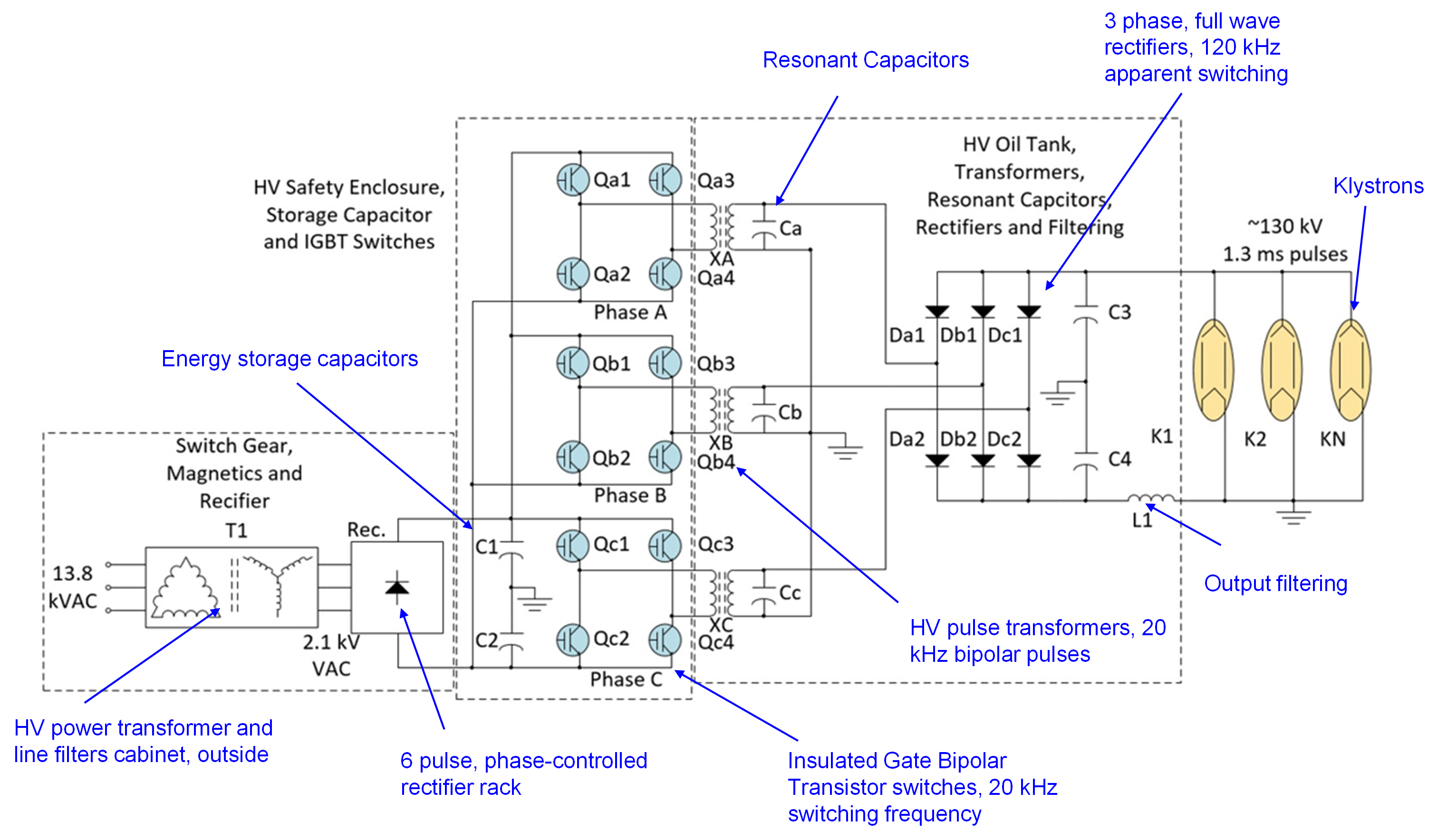
HVCMs are machines powering the linear accelerator klystrons in the accelerator facility. Klystrons produce high-power radio frequency to accelerate negatively charged hydrogen ions. The waveform signals, as shown in the figure below, were collected from the operation of 15 HVCM systems from 2020 to 2022. These datasets contain the waveform signals and the waveform label recorded by the HVCM controller. These binary labels determine if the waveform was collected before a “fault” or “run” (non-fault). Each waveform consists of the 14 signals listed above, the components these originate from in the HVCM are shown in the diagram below the waveform plot. The faults may appear in one or more of these signals, and having one faulty signal is sufficient to label the waveform as faulty. In this benchmark, we ask ML models to correctly classify waveforms from the drift-tube linac (DTL) dataset, one of four datasets provided in Mendeley from [RPW+22].

scheme

Preprocessing

In the following benchmark, we demonstrate pyMAISE on two shapes of data:

Case 1: The raw data is kept as is, with an input shape of \((\text{samples}, \text{time steps}, \text{features})\) and output shape of \((\text{samples}, \text{labels})\).
Case 2: The raw data is stacked following a train/test split to produce an input shape of \((\text{samples}\times \text{time steps}, \text{features})\) and output shape of \((\text{samples} \times \text{time steps}, \text{labels})\) (the labels were propagated out in time for each sample before stacking). We then apply a rolling window with a lookback of 10 to produce an input shape of \((\text{samples} \times \text{time steps} - 9, 10, \text{features})\) and output of \((\text{samples} \times \text{time steps} - 9, 10, \text{labels})\).

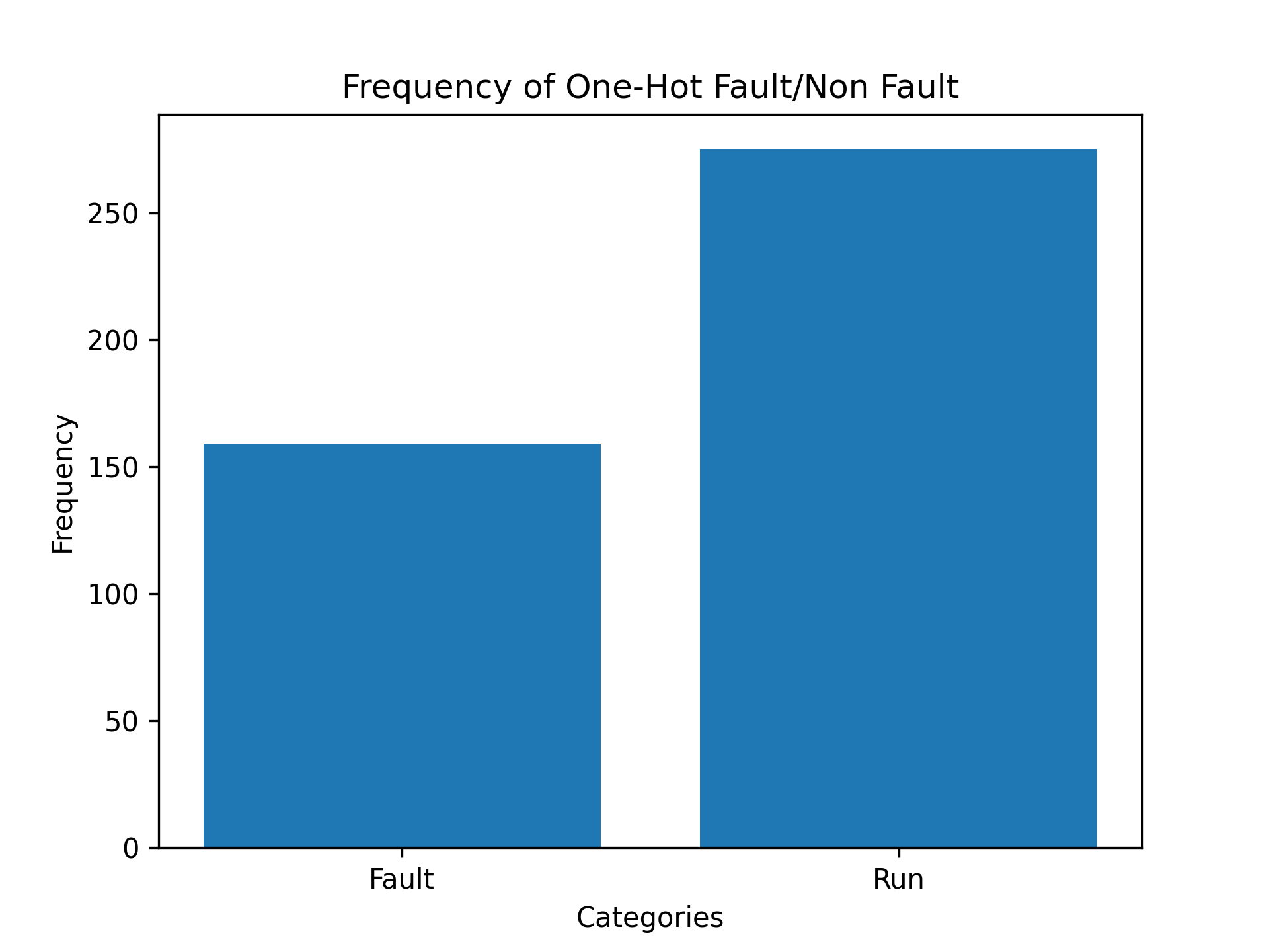
The DTL dataset consists of 1077 waveforms, 159 of which are faulty. To make the classifications more balanced and thus reduce the bias against faulty cases, we randomly cut the number of non-faulty samples to 275 so that 37% of the 434 samples were faulty. This distribution is visualized in the frequency plot below. These samples were randomly split into training and testing sets of sizes 303 and 131, respectively. Each sample consists of 14 features, each characterized by 4500 time steps. The output indicates whether the waveform is faulty or non-faulty and is one-hot encoded. Therefore, the final input and output shapes, including both training and testing sets combined, of each case are

Case 1: input (434, 4500, 14), output (434, 2).
Case 2: input (1952982, 10, 14), output (1952982, 10, 2)

The inputs of each case were min-max scaled.

Frequency of positive/negative values in anomaly detection data.

Hyperparameter Tuning

Given the quantity of data and complexity of the neural networks trained here, we hyperparameter-tuned all models separately. The scripts for hyperparameter tuning these models are provided in the benchmarks/supporting/anomaly/ directory of the pyMAISE GitHub repository. These scripts include the following:

settings.py: This script includes many of the global variables used in this benchmark and the supporting scripts, including:
- input_path: The path to the raw input data taken from Mendeley. Note that we do not host this dataset in pyMAISE as its size is rather large.
- output_path: Path to the labels from Mendeley.
- problem_type = mai.ProblemType.CLASSIFICATION.
- data_random_state = 42: Integer to ensure the data split between Case 1 and 2 is consistent.
- verbosity = 3: Level of output from pyMAISE.
- non_faulty_frac = 0.3: The fraction of “run” or non-faulty data to retain. Non-faulty samples are randomly sampled. Due to the low frequency of “faulty” waveforms, we reduce the total number of “run” waveforms to ensure the models are not overfitting to “run” waveforms.
- test_size = 0.3: The fraction of samples for testing.
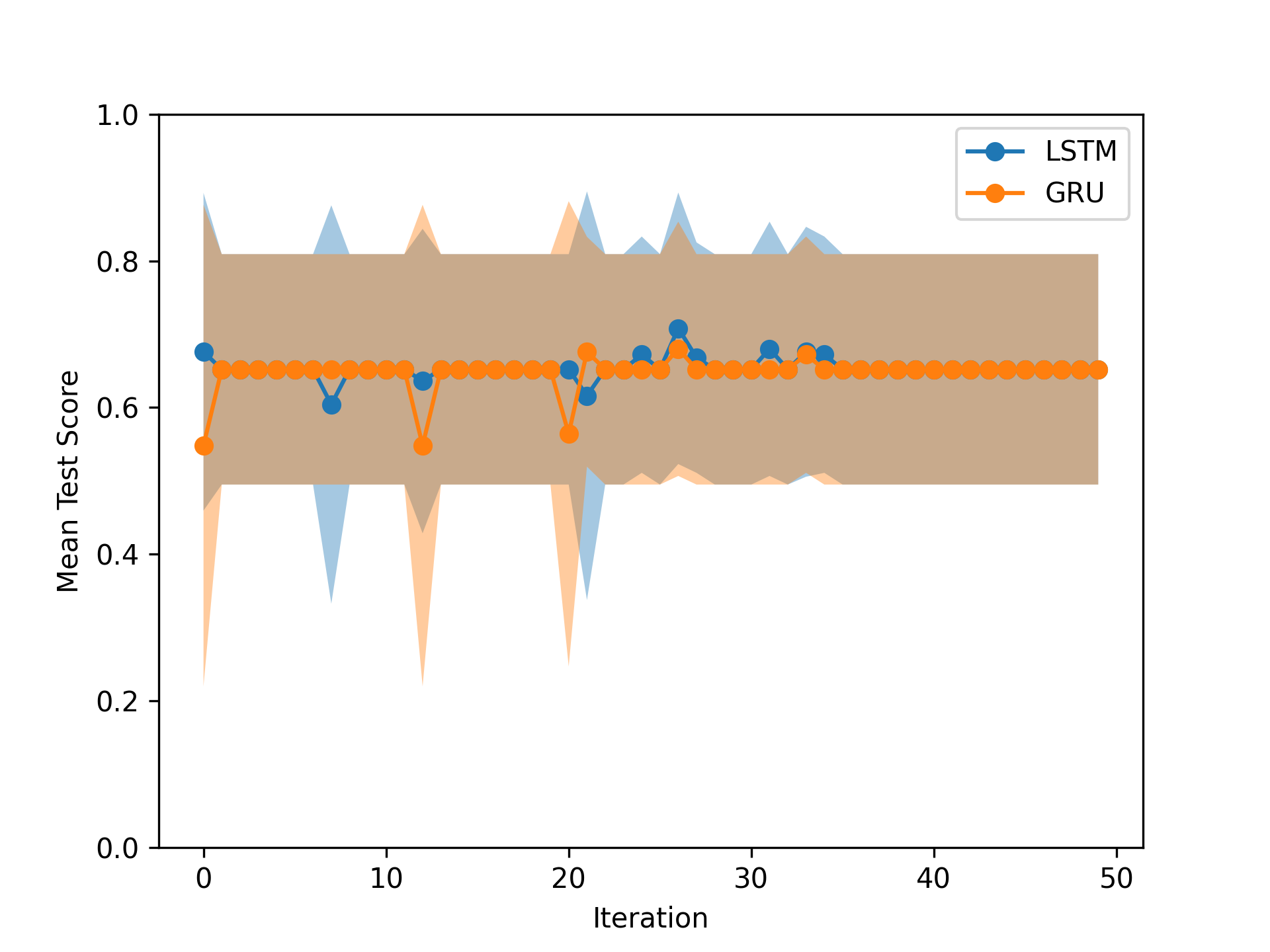
preprocessing.py: A preprocessing script that wraps pyMAISE.datasets.load_anomaly based on the shape of data we desire (Case 1 or 2); this function is load_anomaly_data, and we use it below, too. This function uses the predefined paths in settings.py to load and format the HVCM data. Additionally, we provide a wrapper function for pyMAISE.preprocessing.SplitSequence called split_sequence to utilize pyMAISE-supported functions with the data’s format.
binary_case_1.py: The Hyperparameter tuning script for Case 1 includes the hyperparameter tuning spaces for the LSTM and GRU. Both models are tuned with Bayesian search with 50 iterations of a 5-fold time-series cross-validation split. The results are written to a pickle given at configs/binary_case_1.pkl.
binary_case_2.py: Hyperparameter tuning script for Case 2, which includes the hyperparameter tuning spaces for the LSTM, GRU, and CNN-LSTM. Both models are tuned with Bayesian search with 50 iterations of a 5-fold time-series cross-validation split. The results are written to a pickle given at configs/binary_case_2.pkl.

For the hyperparameter tuning search spaces, please refer to the dictionaries defined in binary_case_1.py and binary_case_2.py, which are defined in typical pyMAISE format.

Postprocessing

Below are the results of Cases 1 and 2. We first load the data using the wrapper functions discussed in the previous section and then load the pickle of hyperparameter configurations. These are then trained again in the pyMAISE.PostProcessor, and we discuss the result.

[1]:

# Import other packages
import pickle
import sys
import numpy as np
import matplotlib.pyplot as plt
sys.path.insert(0, "supporting/anomaly")

# pyMAISE specific imports
from supporting.anomaly.preprocessing import load_anomaly_data, split_sequences
import supporting.anomaly.settings as anomaly_settings
import pyMAISE as mai

# Plot settings
matplotlib_settings = {
    "font.size": 12,
    "legend.fontsize": 12,
    "figure.figsize": (8, 8)
}
plt.rcParams.update(**matplotlib_settings)

[2]:

global_settings = mai.init(
    problem_type=anomaly_settings.problem_type,
    random_state=anomaly_settings.random_state,
    cuda_visible_devices="1",  # Use GPU 1
)

Case 1: 3D Data

We load the DTL dataset using the load_anomaly_data wrapper function implemented in benchmarks/supporting/anomaly/preprocessing.py. The shapes of train/test input/output sets are shown below.

[3]:

xtrain, xtest, ytrain, ytest, xscaler = load_anomaly_data(
    global_settings=global_settings,
    stack_series=False,
    multiclass=False,
    test_size=anomaly_settings.test_size,
    non_faulty_frac=anomaly_settings.non_faulty_frac,
    timestep_step=1,
)
mai._try_clear()

print(f"xtrain shape: {xtrain.shape}")
print(f"ytrain shape: {ytrain.shape}")
print(f"xtest shape: {xtest.shape}")
print(f"ytest shape: {ytest.shape}")

xtrain shape: (303, 4500, 14)
ytrain shape: (303, 2)
xtest shape: (131, 4500, 14)
ytest shape: (131, 2)

[4]:

xtrain

[5]:

ytrain

For Case 1, we hyperparameter-tuned the following models:

Long short-term memory neural network: LSTM,
Gated recurrent unit neural network: GRU,

by running benchmarks/supporting/anomaly/binary_case_1.py. Below is the convergence plot for the Bayesian search.

bc1

To postprocess these models we can load the pickle found at benchmarks/supporting/anomaly/configs/binary_case_1.pkl.

[6]:

with open("supporting/anomaly/configs/binary_case_1.pkl", "rb") as f:
    configs = pickle.load(f)
mai._try_clear()

Model Postprocessing

With the hyperparameter configurations and data, we can retrain the models on the whole dataset using the pyMAISE.PostProcessor. For both models, we increase the epochs from 7 to 100.

[7]:

postprocessor = mai.PostProcessor(
    data=(xtrain, xtest, ytrain, ytest),
    model_configs=[configs],
    new_model_settings={
        "LSTM": {"fitting_params": {"epochs": 100}},
        "GRU": {"fitting_params": {"epochs": 100}},
    },
)

Below are the performance metrics for the two models on this classification problem.

[8]:

postprocessor.metrics().drop("Parameter Configurations", axis=1)

[8]:

	Model Types	Train Accuracy	Train Recall	Train Precision	Train F1	Test Accuracy	Test Recall	Test Precision	Test F1
2	LSTM	0.768977	0.768977	0.768977	0.768977	0.755725	0.755725	0.755725	0.755725
4	LSTM	0.745875	0.745875	0.745875	0.745875	0.679389	0.679389	0.679389	0.679389
6	GRU	0.745875	0.745875	0.745875	0.745875	0.679389	0.679389	0.679389	0.679389
5	GRU	0.739274	0.739274	0.739274	0.739274	0.671756	0.671756	0.671756	0.671756
7	GRU	0.739274	0.739274	0.739274	0.739274	0.671756	0.671756	0.671756	0.671756
8	GRU	0.716172	0.716172	0.716172	0.716172	0.671756	0.671756	0.671756	0.671756
9	GRU	0.726073	0.726073	0.726073	0.726073	0.671756	0.671756	0.671756	0.671756
3	LSTM	0.712871	0.712871	0.712871	0.712871	0.618321	0.618321	0.618321	0.618321
0	LSTM	0.656766	0.656766	0.656766	0.656766	0.580153	0.580153	0.580153	0.580153
1	LSTM	0.564356	0.564356	0.564356	0.564356	0.549618	0.549618	0.549618	0.549618

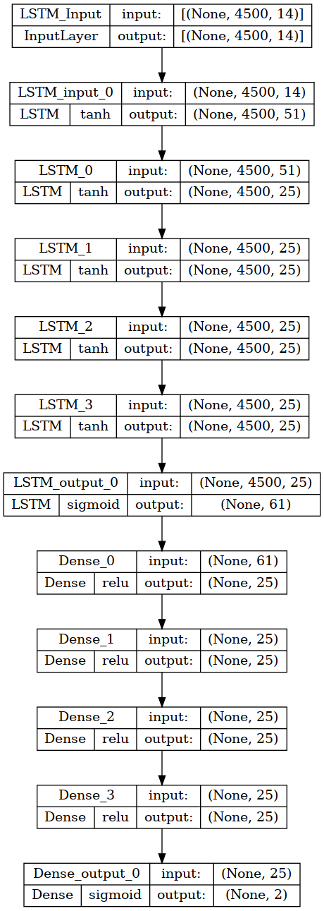
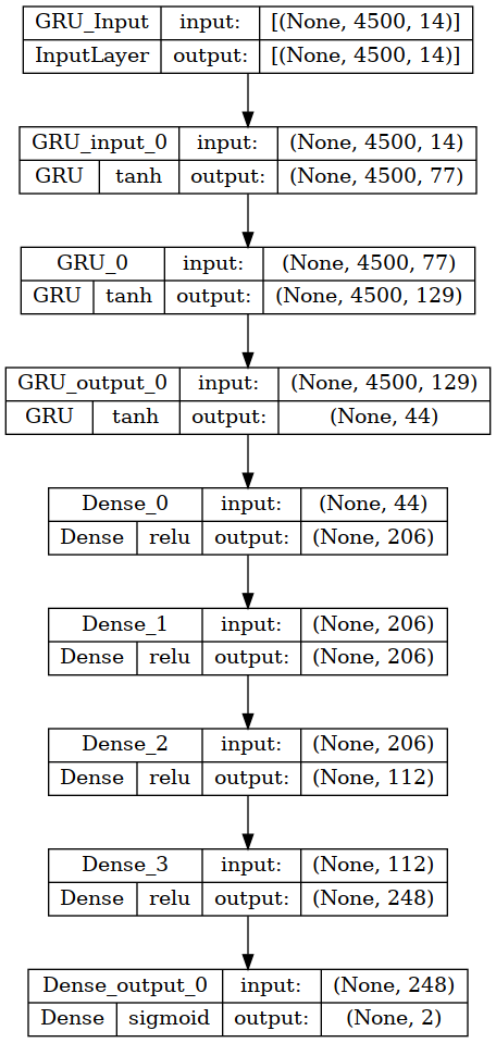
The LSTM outperforms the GRU with a test accuracy close to 0.75. The remaining models overfit the training data. Below, we show the optimal hyperparameters and the network plots for the LSTM and GRU, respectively.

[9]:

for model in ["LSTM", "GRU"]:
    postprocessor.print_model(model_type=model)
    print()

Model Type: LSTM
  Structural Hyperparameters
    Layer: LSTM_input_0
      units: 51
    Layer: LSTM_0
      units: 25
      activation: tanh
    Layer: LSTM_1
      units: 25
      activation: tanh
    Layer: LSTM_2
      units: 25
      activation: tanh
    Layer: LSTM_3
      units: 25
      activation: tanh
    Layer: LSTM_output_0
      units: 61
      activation: sigmoid
    Layer: Dense_0
      units: 25
    Layer: Dense_1
      units: 25
    Layer: Dense_2
      units: 25
    Layer: Dense_3
      units: 25
    Layer: Dense_output_0
  Compile/Fitting Hyperparameters
    Adam_learning_rate: 3.223746051302877e-05
    Adam_clipnorm: 0.9314610424860413
    Adam_clipvalue: 0.5187788874324804
    batch_size: 8
Model: "LSTM"
_________________________________________________________________
 Layer (type)                Output Shape              Param #
=================================================================
 LSTM_input_0 (LSTM)         (None, 4500, 51)          13464

 LSTM_0 (LSTM)               (None, 4500, 25)          7700

 LSTM_1 (LSTM)               (None, 4500, 25)          5100

 LSTM_2 (LSTM)               (None, 4500, 25)          5100

 LSTM_3 (LSTM)               (None, 4500, 25)          5100

 LSTM_output_0 (LSTM)        (None, 61)                21228

 Dense_0 (Dense)             (None, 25)                1550

 Dense_1 (Dense)             (None, 25)                650

 Dense_2 (Dense)             (None, 25)                650

 Dense_3 (Dense)             (None, 25)                650

 Dense_output_0 (Dense)      (None, 2)                 52

=================================================================
Total params: 61244 (239.23 KB)
Trainable params: 61244 (239.23 KB)
Non-trainable params: 0 (0.00 Byte)
_________________________________________________________________

Model Type: GRU
  Structural Hyperparameters
    Layer: GRU_input_0
      units: 77
    Layer: GRU_0
      units: 129
      activation: tanh
    Layer: GRU_output_0
      units: 44
      activation: tanh
    Layer: Dense_0
      units: 206
    Layer: Dense_1
      units: 206
    Layer: Dense_2
      units: 112
    Layer: Dense_3
      units: 248
    Layer: Dense_output_0
  Compile/Fitting Hyperparameters
    Adam_learning_rate: 0.0007461481432054364
    Adam_clipnorm: 0.9696816514952583
    Adam_clipvalue: 0.52238997961519
    batch_size: 32
Model: "GRU"
_________________________________________________________________
 Layer (type)                Output Shape              Param #
=================================================================
 GRU_input_0 (GRU)           (None, 4500, 77)          21483

 GRU_0 (GRU)                 (None, 4500, 129)         80496

 GRU_output_0 (GRU)          (None, 44)                23100

 Dense_0 (Dense)             (None, 206)               9270

 Dense_1 (Dense)             (None, 206)               42642

 Dense_2 (Dense)             (None, 112)               23184

 Dense_3 (Dense)             (None, 248)               28024

 Dense_output_0 (Dense)      (None, 2)                 498

=================================================================
Total params: 228697 (893.35 KB)
Trainable params: 228697 (893.35 KB)
Non-trainable params: 0 (0.00 Byte)
_________________________________________________________________

[10]:

postprocessor.nn_network_plot(
    model_type="LSTM",
    to_file="./supporting/anomaly_lstm_3d.png",
    show_shapes=True,
    show_layer_names=True,
    expand_nested=True,
    show_layer_activations=True,
)

[10]:

[11]:

postprocessor.nn_network_plot(
    model_type="GRU",
    to_file="./supporting/anomaly_gru_3d.png",
    show_shapes=True,
    show_layer_names=True,
    expand_nested=True,
    show_layer_activations=True,
)

[11]:

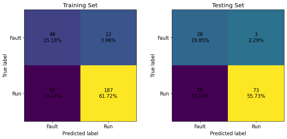
Below we plot the confusion matrices for the LSTM and GRU, respectively.

[12]:

fig, axs = plt.subplots(1, 2, figsize=(12, 5))
postprocessor.confusion_matrix(axs=axs, model_type="LSTM")
plt.show()

[13]:

fig, axs = plt.subplots(1, 2, figsize=(12, 5))
postprocessor.confusion_matrix(axs=axs, model_type="GRU")
plt.show()

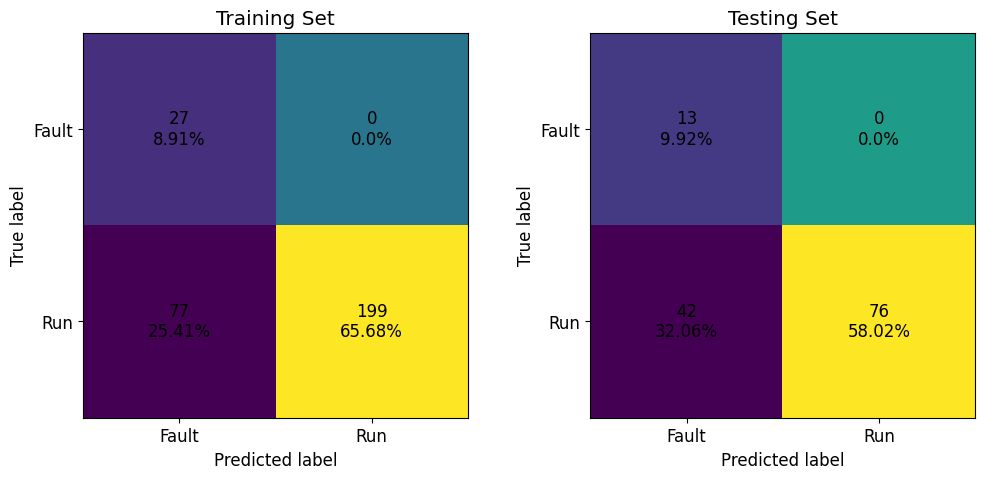
Both models perform well in identifying the non-faulty waveforms; however, they considerably incorrectly classify the faulty waveforms as non-faulty. This may be a feature of the slight bias of the data to the non-faulty waveforms.

Below are the learning curves for both models.

[14]:

models = np.array([["LSTM", "GRU"]])
fig, axarr = plt.subplots(models.shape[0], models.shape[1], sharex=True, sharey=True, figsize=(12,6))
for i in range(models.shape[1]):
    plt.sca(axarr[i])
    axarr[i] = postprocessor.nn_learning_plot(model_type=models[0, i])
    axarr[i].set_title(models[0, i])
plt.show()

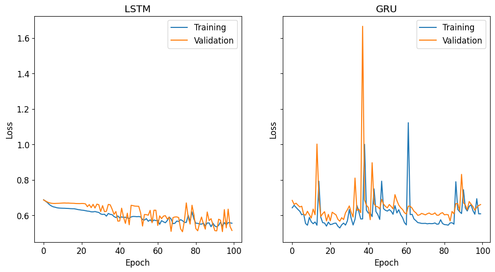
We see that minimizing the cross-entropy includes a slight overfitting of the training data for both models. The GRU includes several epochs with sporadically large cross-entropy.

Case 2: 2D Data

We load the DTL dataset using the load_anomaly_data wrapper function implemented in benchmarks/supporting/anomaly/preprocessing.py. The shapes of train/test input/output sets are shown below. We then apply a split sequence using the split_sequence wrapper with a lookback of 10.

[15]:

data = load_anomaly_data(
    global_settings=global_settings,
    stack_series=True,
    multiclass=False,
    test_size=anomaly_settings.test_size,
    non_faulty_frac=anomaly_settings.non_faulty_frac,
    timestep_step=1,
)
xtrain, xtest, ytrain, ytest = split_sequences(
    data=data[:-1],
    input_steps=10,
    output_steps=1,
    output_position=0,
)
mai._try_clear()

print(f"xtrain shape: {xtrain.shape}")
print(f"ytrain shape: {ytrain.shape}")
print(f"xtest shape: {xtest.shape}")
print(f"ytest shape: {ytest.shape}")

xtrain shape: (1363491, 10, 14)
ytrain shape: (1363491, 2)
xtest shape: (589491, 10, 14)
ytest shape: (589491, 2)

[16]:

xtrain

[17]:

ytrain

For Case 2, we hyperparameter-tuned the following models:

Long short-term memory neural network: LSTM,
Gated recurrent unit neural network: GRU,
Convolutional/LSTM neural network: CNN-LSTM,

by running benchmarks/supporting/anomaly/binary_case_2.py. Below is the convergence plot for the Bayesian search.

bc2

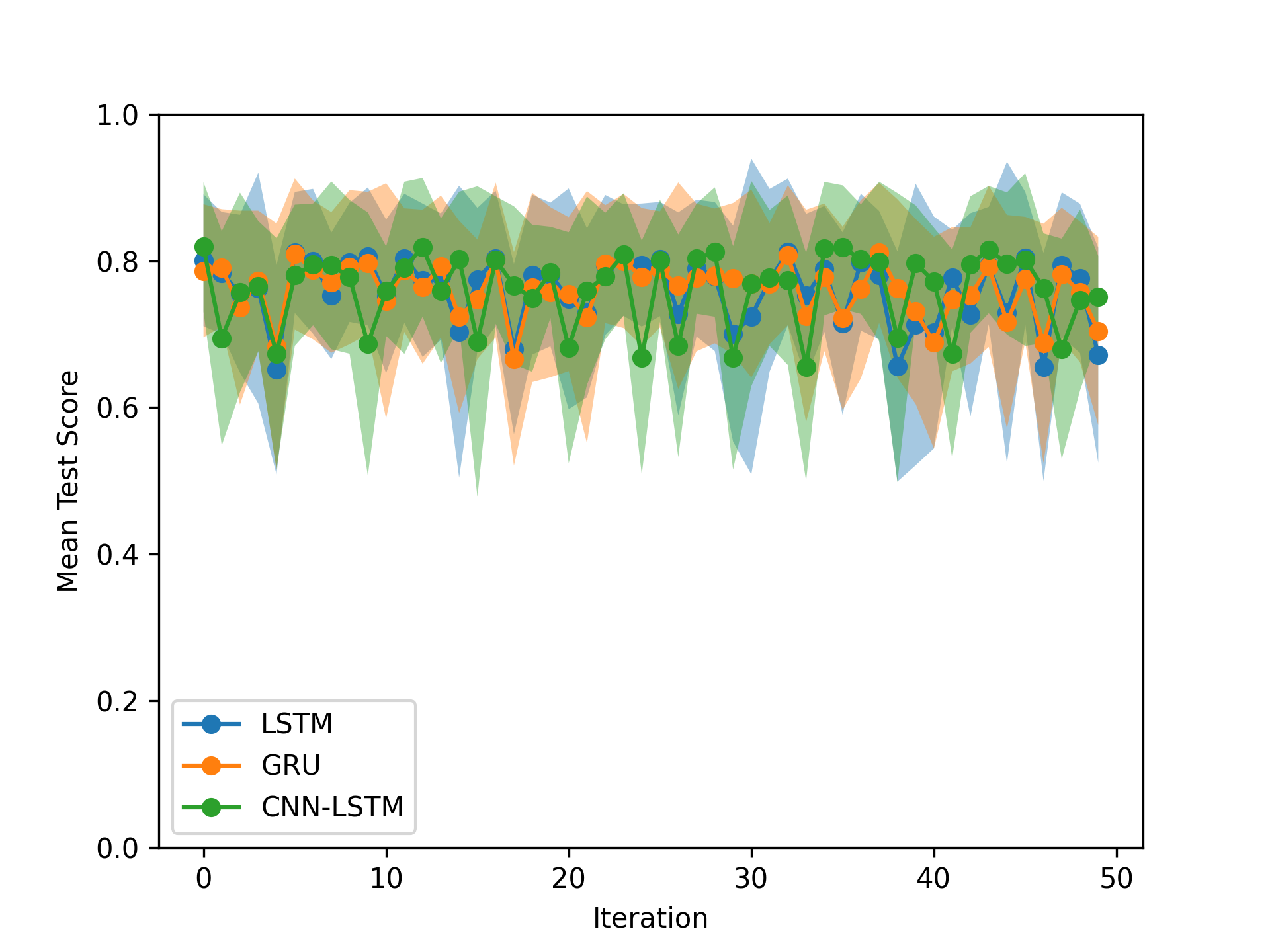
All models perform better in hyperparameter tuning using the data format of Case 2 than Case 1. To postprocess these models, we can load the pickle found at benchmarks/supporting/anomaly/configs/binary_case_2.pkl.

[18]:

with open("supporting/anomaly/configs/binary_case_2.pkl", "rb") as f:
    configs = pickle.load(f)
mai._try_clear()

Model Postprocessing

With the hyperparameter configurations and data, we can retrain the models on the whole dataset using the pyMAISE.PostProcessor. For both models, we increase the epochs from 7 to 30.

[19]:

postprocessor = mai.PostProcessor(
    data=(xtrain, xtest, ytrain, ytest),
    model_configs=[configs],
    new_model_settings={
        "LSTM": {"fitting_params": {"epochs": 30}},
        "GRU": {"fitting_params": {"epochs": 30}},
        "CNN-LSTM": {"fitting_params": {"epochs": 30}},
    },
)

Below are the performance metrics for the two models on this classification problem.

[20]:

postprocessor.metrics().drop("Parameter Configurations", axis=1)

[20]:

	Model Types	Train Accuracy	Train Recall	Train Precision	Train F1	Test Accuracy	Test Recall	Test Precision	Test F1
10	CNN-LSTM	0.841929	0.841929	0.841929	0.841929	0.805956	0.805956	0.805956	0.805956
3	LSTM	0.843386	0.843386	0.843386	0.843386	0.800153	0.800153	0.800153	0.800153
11	CNN-LSTM	0.844380	0.844380	0.844380	0.844380	0.798574	0.798574	0.798574	0.798574
2	LSTM	0.842965	0.842965	0.842965	0.842965	0.797493	0.797493	0.797493	0.797493
6	GRU	0.841691	0.841691	0.841691	0.841691	0.796277	0.796277	0.796277	0.796277
9	GRU	0.838020	0.838020	0.838020	0.838020	0.796046	0.796046	0.796046	0.796046
8	GRU	0.847015	0.847015	0.847015	0.847015	0.794119	0.794119	0.794119	0.794119
4	LSTM	0.843840	0.843840	0.843840	0.843840	0.793547	0.793547	0.793547	0.793547
1	LSTM	0.841962	0.841962	0.841962	0.841962	0.793001	0.793001	0.793001	0.793001
14	CNN-LSTM	0.840165	0.840165	0.840165	0.840165	0.792638	0.792638	0.792638	0.792638
7	GRU	0.844850	0.844887	0.844856	0.844871	0.792552	0.792552	0.792552	0.792552
0	LSTM	0.842399	0.842399	0.842399	0.842399	0.789656	0.789656	0.789656	0.789656
5	GRU	0.845931	0.845931	0.845931	0.845931	0.789576	0.789576	0.789576	0.789576
12	CNN-LSTM	0.839651	0.839651	0.839651	0.839651	0.784280	0.784280	0.784280	0.784280
13	CNN-LSTM	0.703837	0.703837	0.703837	0.703837	0.684139	0.684139	0.684139	0.684139

The LSTM, GRU, and CNN-LSTM all perform within 0.01 test accuracy of each other, showing a higher degree of generalizability to unseen data than the produced in Case 1. Additionally, all metrics are considerably better than Case 1.

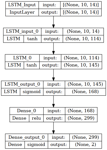
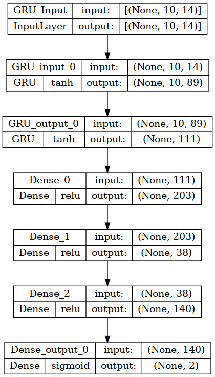
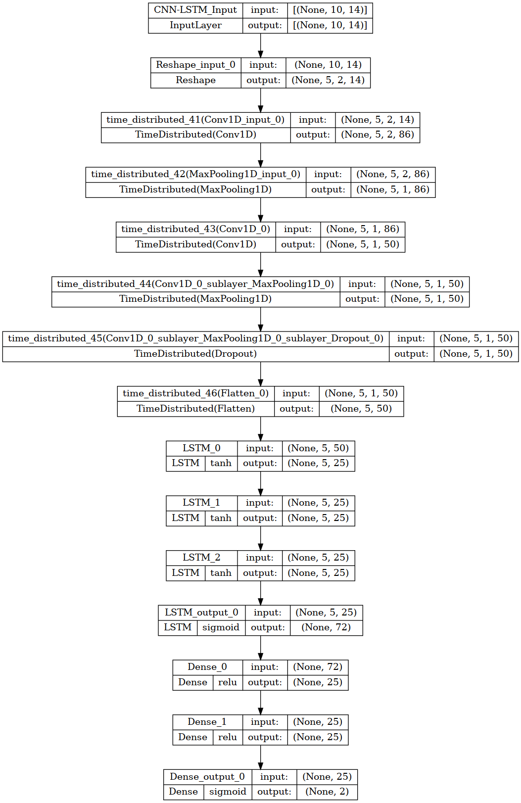
Below are the optimal hyperparameter configurations and network plots for the LSTM, GRU, and CNN-LSTM, respectively.

[21]:

for model in ["LSTM", "GRU", "CNN-LSTM"]:
    postprocessor.print_model(model_type=model)
    print()

Model Type: LSTM
  Structural Hyperparameters
    Layer: LSTM_input_0
      units: 114
    Layer: LSTM_0
      units: 145
      activation: tanh
    Layer: LSTM_output_0
      units: 168
      activation: sigmoid
    Layer: Dense_0
      units: 299
    Layer: Dense_output_0
  Compile/Fitting Hyperparameters
    Adam_learning_rate: 0.00010123356602102984
    Adam_clipnorm: 0.915016200236164
    Adam_clipvalue: 0.3648201326572756
    batch_size: 32
Model: "LSTM"
_________________________________________________________________
 Layer (type)                Output Shape              Param #
=================================================================
 LSTM_input_0 (LSTM)         (None, 10, 114)           58824

 LSTM_0 (LSTM)               (None, 10, 145)           150800

 LSTM_output_0 (LSTM)        (None, 168)               211008

 Dense_0 (Dense)             (None, 299)               50531

 Dense_output_0 (Dense)      (None, 2)                 600

=================================================================
Total params: 471763 (1.80 MB)
Trainable params: 471763 (1.80 MB)
Non-trainable params: 0 (0.00 Byte)
_________________________________________________________________

Model Type: GRU
  Structural Hyperparameters
    Layer: GRU_input_0
      units: 89
    Layer: GRU_output_0
      units: 111
      activation: tanh
    Layer: Dense_0
      units: 203
    Layer: Dense_1
      units: 38
    Layer: Dense_2
      units: 140
    Layer: Dense_output_0
  Compile/Fitting Hyperparameters
    Adam_learning_rate: 5.789366390963926e-05
    Adam_clipnorm: 1.198217983947213
    Adam_clipvalue: 0.39043949470905037
    batch_size: 32
Model: "GRU"
_________________________________________________________________
 Layer (type)                Output Shape              Param #
=================================================================
 GRU_input_0 (GRU)           (None, 10, 89)            28035

 GRU_output_0 (GRU)          (None, 111)               67266

 Dense_0 (Dense)             (None, 203)               22736

 Dense_1 (Dense)             (None, 38)                7752

 Dense_2 (Dense)             (None, 140)               5460

 Dense_output_0 (Dense)      (None, 2)                 282

=================================================================
Total params: 131531 (513.79 KB)
Trainable params: 131531 (513.79 KB)
Non-trainable params: 0 (0.00 Byte)
_________________________________________________________________

Model Type: CNN-LSTM
  Structural Hyperparameters
    Layer: Reshape_input_0
    Layer: time_distributed_35
    Layer: time_distributed_36
    Layer: time_distributed_37
    Layer: time_distributed_38
    Layer: time_distributed_39
    Layer: time_distributed_40
    Layer: LSTM_0
      units: 25
      activation: tanh
      recurrent_dropout: 0.0
    Layer: LSTM_1
      units: 25
      activation: tanh
      recurrent_dropout: 0.0
    Layer: LSTM_2
      units: 25
      activation: tanh
      recurrent_dropout: 0.0
    Layer: LSTM_output_0
      units: 72
      activation: sigmoid
    Layer: Dense_0
      units: 25
    Layer: Dense_1
      units: 25
    Layer: Dense_output_0
  Compile/Fitting Hyperparameters
    Adam_learning_rate: 0.0002068402637884372
    Adam_clipnorm: 0.8824961730815847
    Adam_clipvalue: 0.3422836801045622
    batch_size: 32
Model: "CNN-LSTM"
_________________________________________________________________
 Layer (type)                Output Shape              Param #
=================================================================
 Reshape_input_0 (Reshape)   (None, 5, 2, 14)          0

 time_distributed_35 (TimeD  (None, 5, 2, 86)          2494
 istributed)

 time_distributed_36 (TimeD  (None, 5, 1, 86)          0
 istributed)

 time_distributed_37 (TimeD  (None, 5, 1, 50)          4350
 istributed)

 time_distributed_38 (TimeD  (None, 5, 1, 50)          0
 istributed)

 time_distributed_39 (TimeD  (None, 5, 1, 50)          0
 istributed)

 time_distributed_40 (TimeD  (None, 5, 50)             0
 istributed)

 LSTM_0 (LSTM)               (None, 5, 25)             7600

 LSTM_1 (LSTM)               (None, 5, 25)             5100

 LSTM_2 (LSTM)               (None, 5, 25)             5100

 LSTM_output_0 (LSTM)        (None, 72)                28224

 Dense_0 (Dense)             (None, 25)                1825

 Dense_1 (Dense)             (None, 25)                650

 Dense_output_0 (Dense)      (None, 2)                 52

=================================================================
Total params: 55395 (216.39 KB)
Trainable params: 55395 (216.39 KB)
Non-trainable params: 0 (0.00 Byte)
_________________________________________________________________

[22]:

postprocessor.nn_network_plot(
    model_type="LSTM",
    to_file="./supporting/anomaly_lstm_2d.png",
    show_shapes=True,
    show_layer_names=True,
    expand_nested=True,
    show_layer_activations=True,
)

[22]:

[23]:

postprocessor.nn_network_plot(
    model_type="GRU",
    to_file="./supporting/anomaly_gru_2d.png",
    show_shapes=True,
    show_layer_names=True,
    expand_nested=True,
    show_layer_activations=True,
)

[23]:

[24]:

postprocessor.nn_network_plot(
    model_type="CNN-LSTM",
    to_file="./supporting/anomaly_cnnlstm_2d.png",
    show_shapes=True,
    show_layer_names=True,
    expand_nested=True,
    show_layer_activations=True,
)

[24]:

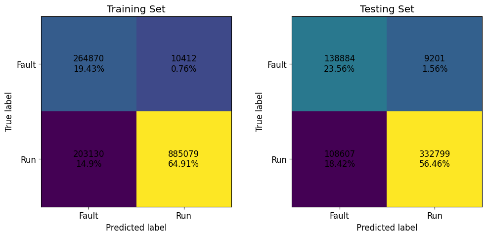
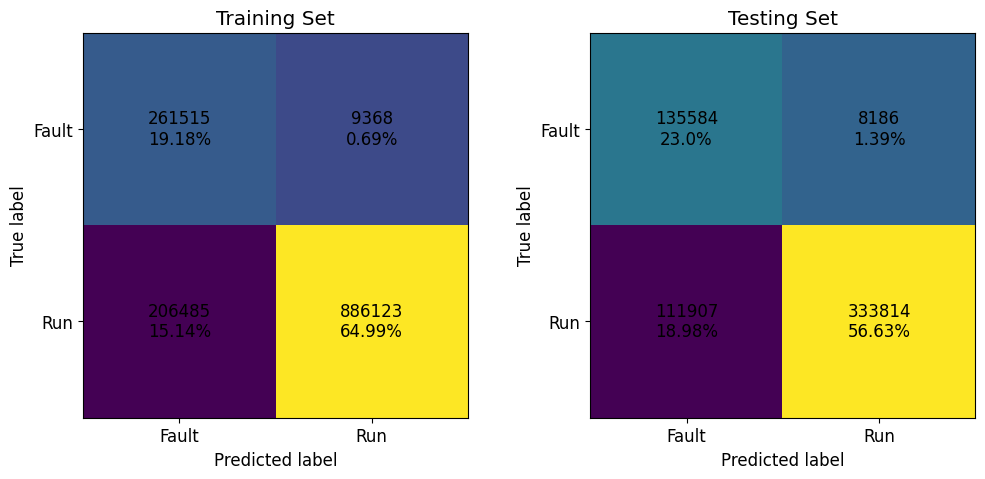
Below we plot the confusion matrices for the LSTM, GRU, and CNN-LSTM, respectively.

[25]:

fig, axs = plt.subplots(1, 2, figsize=(12, 5))
postprocessor.confusion_matrix(axs=axs, model_type="LSTM")
plt.show()

[26]:

fig, axs = plt.subplots(1, 2, figsize=(12, 5))
postprocessor.confusion_matrix(axs=axs, model_type="GRU")
plt.show()

[27]:

fig, axs = plt.subplots(1, 2, figsize=(12, 5))
postprocessor.confusion_matrix(axs=axs, model_type="CNN-LSTM")
plt.show()

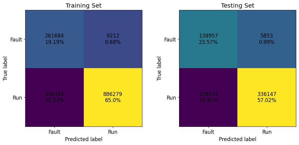
The resulting percentages follow that shown in Case 1; however, the percentage of faulty waveforms misclassified was reduced by more than 5%.

Below are the learning curves.

[28]:

models = np.array([["LSTM", "GRU"]])
fig = plt.figure(figsize=(12, 12))
gs = fig.add_gridspec(2, 2)
for i in range(models.shape[0]):
    for j in range(models.shape[1]):
        ax = fig.add_subplot(gs[i, j])
        ax = postprocessor.nn_learning_plot(model_type=models[i, j])
        ax.set_title(models[i, j])
ax = fig.add_subplot(gs[1, :])
ax = postprocessor.nn_learning_plot(model_type="CNN-LSTM")
ax.set_title("CNN-LSTM")
plt.show()

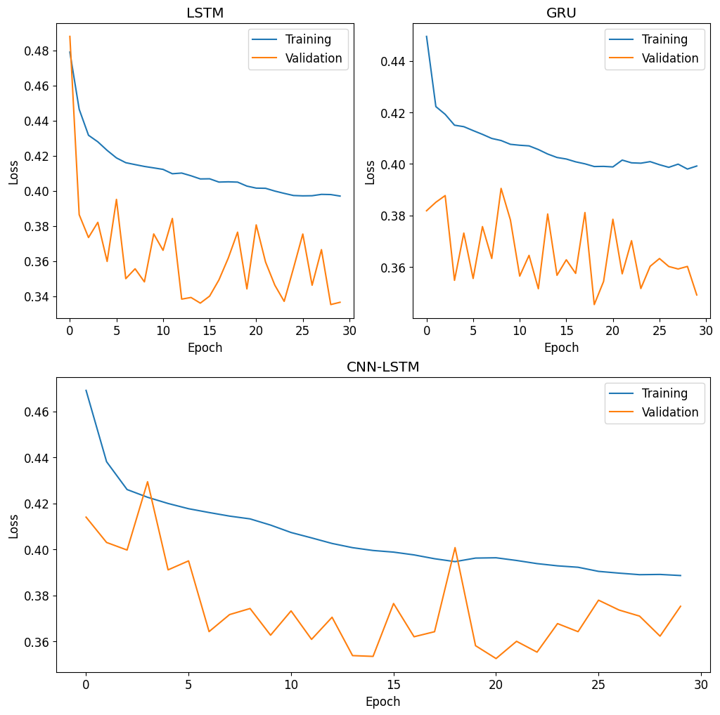
The learning curves for all three models indicate they are not overfitting the training set. Additionally, their convergence is much more predictable.