Fuel Performance

Inputs

fuel_dens: Fuel density (\(\frac{kg}{m^3}\))
porosity: Porosity
clad_thick: Cladding thickness (\(m\))
pellet_OD: Pellet outer diameter (\(m\))
pellet_h: Pellet height (\(m\))
gap_thick: Gap thickness (\(m\))
inlet_T: Inlet temperature (\(K\))
enrich: U-235 enrichment
rough_fuel: Fuel roughness (\(m\))
rough_clad: Clad roughness (\(m\))
ax_pow: Axial power
clad_T: Cladding surface temperature (\(K\))
pressure: Pressure (\(Pa\))

Outputs

fis_gas_produced: Fission gas production (\(mol\))
max_fuel_centerline_temp: Max fuel centerline temperature (\(K\))
max_fuel_surface_temp: Max fuel surface temperature (\(K\))
radial_clad_dia: Radial cladding diameter displacement after irradiation (\(m\))

This data set comprises 13 inputs and four outputs with 400 data points. This data originates from [RK20], and a graphical representation is provided in the figure below. Case 1 from the pellet-cladding mechanical interaction (PCMI) benchmark was selected for the data set. This benchmark simulates a beginning of life (BOL) ramp of a 10-pellet pressurized water reactor (PWR) fuel rod to an average linear heat rate of \(40~kW/m\). The inner and outer cladding diameters are reduced, so the fuel-clad interaction occurs during the ramp time. Axial power and rod surface temperature profiles were assumed to be uniform at \(330^\circ C\). The 13 input parameters were uniformly randomly sampled independently within their uncertainty bounds and simulated in BISON. The rod response was recorded in 4 outputs.

The following are a few common packages and functions that will prove useful while using pyMAISE along with pyMAISE-specific functionality.

[1]:

%load_ext autoreload
%autoreload 2

# Importing Packages
import time
import cv2
import numpy as np
import matplotlib.pyplot as plt
from scipy.stats import uniform, randint
from sklearn.preprocessing import MinMaxScaler

# pyMAISE specific imports
import pyMAISE as mai
from pyMAISE.datasets import load_fp
from pyMAISE.preprocessing import scale_data, train_test_split, correlation_matrix

# Plot settings
matplotlib_settings = {
    "font.size": 12,
    "legend.fontsize": 11,
    "figure.figsize": (8, 8)
}
plt.rcParams.update(**matplotlib_settings)

Model Initialization

We will examine the performance of six models in this data set:

Linear regression: Linear,
Lasso regression: Lasso,
Decision tree regression: DT,
Random forest regression: RF,
K-nearest neighbors regression: KN,
Sequential dense neural networks: FNN.

For hyper-parameter tuning each model, we must initialize the architecture and optimize search spaces.

[7]:

# Initializing all the models wanted along with neurel network archetecture/optimization hps
model_settings = {
    "models": ["Linear", "Lasso", "DT", "RF", "KN", "FNN"],
    "FNN": {
        "structural_params": {
            "Dense_hidden": {
                "num_layers": mai.Int(min_value=0, max_value=2),
                "units": mai.Int(min_value=25, max_value=400),
                "activation": "relu",
                "kernel_initializer": "normal",
                "sublayer": mai.Choice(["Dropout_hidden", "None"]),
                "Dropout_hidden": {
                    "rate": mai.Float(min_value=0.2, max_value=0.6),
                },
            },
            "Dense_output": {
                "units": ytrain.shape[-1],
                "activation": "linear",
                "kernel_initializer": "normal",
            },
        },
        "optimizer": "Adam",
        "Adam": {
            "learning_rate": mai.Float(min_value=1e-5, max_value=0.001),
        },
        "compile_params": {
            "loss": "mean_absolute_error",
            "metrics": ["mean_absolute_error"],
        },
        "fitting_params": {
            "batch_size": mai.Choice([8, 16, 32]),
            "epochs": 50,
            "validation_split": 0.15,
        },
    },
}
# Constructing Tuner object for the search space above
tuner = mai.Tuner(xtrain, ytrain, model_settings=model_settings)

Hyperparameter Tuning

We will use random search for the hyperparameter tuning of the classical models (Lasso, DT, RF, and KN) through the pyMAISE.Tuner.random_search function. Linear will be manually fit with the Scikit-learn defaults. Three hundred models will be produced with randomly sampled parameter configurations for each classical model. For FNN, Bayesian search optimizes the hyper-parameters in 50 iterations through the pyMAISE.Tuner.nn_bayesian_search function. Bayesian search is appealing for FNNs as their training can be computationally expensive. To further reduce the computational cost of FNN, we specify only 10 epochs, which will produce less than performant models but show the optimal parameters. For both search methods, we use cross-validation to reduce bias in the models from the data set. The random_search_spaces and bayesian_search_spaces dictionaries define the hyperparameter search spaces.

[8]:

# Classical Model search space
random_search_spaces = {
    "Lasso": {
        "alpha": uniform(loc=0.0001, scale=0.0099), # 0.0001 - 0.01
    },
    "DT": {
        "max_depth": randint(low=5, high=50), # 5 - 50
        "max_features": [None, "sqrt", "log2", 2, 4, 6],
        "min_samples_split": randint(low=2, high=20), # 2 - 20
        "min_samples_leaf": randint(low=1, high=20), # 1 - 20
    },
    "RF": {
        "n_estimators": randint(low=50, high=200), # 50 - 200
        "criterion": ["squared_error", "absolute_error", "poisson"],
        "min_samples_split": randint(low=2, high=20), # 2 - 20
        "min_samples_leaf": randint(low=1, high=20), # 1 - 20
        "max_features": [None, "sqrt", "log2", 2, 4, 6],
    },
    "KN": {
        "n_neighbors": randint(low=1, high=20), # 1 - 20
        "weights": ["uniform", "distance"],
        "leaf_size": randint(low=1, high=30), # 1 - 30
        "p": randint(low=1, high=10), # 1 - 10
    },
}

start = time.time()
random_search_configs = tuner.random_search(
    param_spaces=random_search_spaces,
    n_iter=300,
    n_jobs=6,
    cv=5,
)
bayesian_search_configs = tuner.nn_bayesian_search(
    objective="r2_score",
    max_trials=50,
    cv=5,
)
print("Hyperparameter tuning took " + str((time.time() - start) / 60) + " minutes to process.")

Hyperparameter tuning took 18.119175509611765 minutes to process.

We can understand the hyperparameter tuning of Bayesian search from the convergence plot.

[9]:

ax = tuner.convergence_plot(model_types="FNN")
ax.set_ylim([0, 1])
plt.show()

../_images/benchmarks_fuel_performance_17_0.png

Model Postprocessing

Now that the top pyMAISE.Settings.num_configs_saved is saved, we can pass these models to the pyMAISE.PostProcessor for model comparison and analysis. We can pass an updated epoch parameter to improve the FNN performance. Using 200 epochs should improve fitting at a higher computational cost.

[10]:

postprocessor = mai.PostProcessor(
    data=(xtrain, xtest, ytrain, ytest),
    model_configs=[random_search_configs, bayesian_search_configs],
    new_model_settings={
        "FNN": {"fitting_params": {"epochs": 200}},
    },
    yscaler=yscaler,
)

To compare the performance of these models, we compute 5 regression metrics for both the training and testing data starting with fis_gas_produced.

[11]:

postprocessor.metrics(y="fis_gas_produced").drop("Parameter Configurations", axis=1)

[11]:

	Model Types	Train R2	Train MAE	Train MAPE	Train RMSE	Train RMSPE	Test R2	Test MAE	Test MAPE	Test RMSE	Test RMSPE
2	Lasso	0.999187	3.351089e-08	0.107147	4.154574e-08	0.131630	0.999282	3.335318e-08	0.108170	4.174585e-08	0.135973
1	Lasso	0.999180	3.358087e-08	0.107335	4.170268e-08	0.132012	0.999278	3.340049e-08	0.108290	4.183685e-08	0.136205
0	Linear	0.999248	3.194073e-08	0.102551	3.995663e-08	0.128162	0.999251	3.442157e-08	0.112070	4.261348e-08	0.139910
3	Lasso	0.999089	3.480072e-08	0.110765	4.397708e-08	0.137715	0.999200	3.494171e-08	0.112790	4.405997e-08	0.142598
4	Lasso	0.999087	3.481969e-08	0.110821	4.400934e-08	0.137802	0.999199	3.496989e-08	0.112877	4.409416e-08	0.142700
5	Lasso	0.999002	3.594270e-08	0.114137	4.602351e-08	0.143395	0.999118	3.660263e-08	0.117959	4.624373e-08	0.149225
21	FNN	0.999025	3.733452e-08	0.120502	4.549479e-08	0.147288	0.998740	4.386864e-08	0.141990	5.527846e-08	0.179529
25	FNN	0.998457	4.676055e-08	0.150498	5.722408e-08	0.184242	0.998366	4.870615e-08	0.157073	6.295917e-08	0.201153
23	FNN	0.998732	4.116140e-08	0.131734	5.187295e-08	0.165737	0.998108	5.252240e-08	0.170993	6.775068e-08	0.223516
22	FNN	0.998698	4.052280e-08	0.130647	5.255777e-08	0.170359	0.997971	5.184415e-08	0.168386	7.015318e-08	0.231091
24	FNN	0.996386	8.184828e-08	0.264032	8.756476e-08	0.283359	0.995493	9.203348e-08	0.300544	1.045676e-07	0.344222
11	RF	0.940100	2.270330e-07	0.736522	3.565085e-07	1.178223	0.822613	3.718841e-07	1.221562	6.559852e-07	2.176629
14	RF	0.911887	2.781126e-07	0.901259	4.323916e-07	1.422290	0.801043	3.959614e-07	1.299350	6.947238e-07	2.308605
12	RF	0.970167	1.685515e-07	0.544894	2.515990e-07	0.822530	0.800913	4.181856e-07	1.370478	6.949505e-07	2.312095
13	RF	0.979137	1.469470e-07	0.474111	2.104010e-07	0.684878	0.799408	4.367444e-07	1.427533	6.975731e-07	2.311210
15	RF	0.922210	2.714525e-07	0.879088	4.062755e-07	1.334821	0.785965	4.508824e-07	1.476926	7.205682e-07	2.385251
10	DT	0.784018	5.226181e-07	1.680214	6.769645e-07	2.188798	0.714201	6.119823e-07	1.994128	8.326510e-07	2.736402
7	DT	0.784326	5.244259e-07	1.689262	6.764816e-07	2.189315	0.703764	6.167656e-07	2.012717	8.477193e-07	2.792672
8	DT	0.781418	5.305640e-07	1.708917	6.810273e-07	2.203979	0.701854	6.198605e-07	2.023013	8.504478e-07	2.802257
9	DT	0.767248	5.550179e-07	1.791455	7.027553e-07	2.286978	0.694458	6.318360e-07	2.066556	8.609305e-07	2.844667
16	KN	0.771541	5.550595e-07	1.783920	6.962449e-07	2.234611	0.694057	6.777778e-07	2.207377	8.614963e-07	2.818895
6	DT	0.793849	5.043749e-07	1.628892	6.613778e-07	2.147139	0.694046	6.326584e-07	2.062317	8.615117e-07	2.835354
19	KN	0.758388	5.732143e-07	1.842104	7.160066e-07	2.298252	0.690802	6.764286e-07	2.200439	8.660666e-07	2.824367
20	KN	0.758388	5.732143e-07	1.842104	7.160066e-07	2.298252	0.690802	6.764286e-07	2.200439	8.660666e-07	2.824367
17	KN	1.000000	0.000000e+00	0.000000	0.000000e+00	0.000000	0.674003	7.084409e-07	2.302775	8.892823e-07	2.894971
18	KN	1.000000	0.000000e+00	0.000000	0.000000e+00	0.000000	0.664064	7.146616e-07	2.321866	9.027366e-07	2.935249

Fission gas production is well modeled by linear regression, lasso regression, and the FNNs. Random forest, decision tree, and k-nearest neighbors overfit.

[12]:

postprocessor.metrics(y="max_fuel_centerline_temp").drop("Parameter Configurations", axis=1)

[12]:

	Model Types	Train R2	Train MAE	Train MAPE	Train RMSE	Train RMSPE	Test R2	Test MAE	Test MAPE	Test RMSE	Test RMSPE
25	FNN	0.998165	1.236718	0.077523	1.560398	0.097291	0.998552	1.257878	0.078870	1.527746	0.095339
1	Lasso	0.996489	1.752604	0.109593	2.158117	0.134017	0.997437	1.684734	0.105701	2.032226	0.127288
2	Lasso	0.996507	1.748999	0.109369	2.152533	0.133695	0.997437	1.685811	0.105774	2.032363	0.127329
0	Linear	0.996629	1.722046	0.107731	2.114515	0.131667	0.997332	1.729008	0.108565	2.073786	0.130380
3	Lasso	0.996147	1.815523	0.113533	2.260748	0.140096	0.997324	1.726275	0.108265	2.076736	0.129634
4	Lasso	0.996143	1.816214	0.113577	2.261996	0.140171	0.997322	1.727184	0.108321	2.077668	0.129688
5	Lasso	0.995871	1.859314	0.116296	2.340367	0.144910	0.997153	1.787680	0.112075	2.142153	0.133530
23	FNN	0.998997	0.855958	0.053875	1.153409	0.073283	0.996884	1.455507	0.092206	2.241133	0.144278
24	FNN	0.998424	1.102629	0.068953	1.445802	0.090275	0.996861	1.867520	0.117527	2.249145	0.141642
21	FNN	0.998610	1.109020	0.069902	1.357957	0.085810	0.996727	1.921365	0.120872	2.296744	0.144540
22	FNN	0.998887	0.782986	0.049233	1.215199	0.077050	0.996231	1.798486	0.113969	2.464607	0.158097
12	RF	0.961994	5.277740	0.330831	7.100452	0.443626	0.760444	14.501486	0.911324	19.648978	1.229390
13	RF	0.968733	4.904080	0.307620	6.440221	0.402797	0.753433	15.214105	0.955804	19.934439	1.246561
11	RF	0.918919	7.550692	0.473686	10.370965	0.648506	0.730819	15.508138	0.974906	20.828546	1.304867
15	RF	0.921257	7.755574	0.486716	10.220338	0.638317	0.726813	15.698889	0.986602	20.982958	1.313853
14	RF	0.891750	9.064505	0.569038	11.983253	0.750269	0.722797	15.712007	0.987578	21.136640	1.324375
18	KN	1.000000	0.000000	0.000000	0.000000	0.000000	0.687487	18.131641	1.138529	22.442492	1.403003
17	KN	1.000000	0.000000	0.000000	0.000000	0.000000	0.679749	17.819132	1.118023	22.718627	1.418494
16	KN	0.769263	14.278049	0.895759	17.495176	1.094843	0.676550	18.125236	1.137420	22.831796	1.424511
19	KN	0.754447	14.535587	0.912056	18.048136	1.130196	0.664443	18.220772	1.143238	23.255199	1.450344
20	KN	0.754447	14.535587	0.912056	18.048136	1.130196	0.664443	18.220772	1.143238	23.255199	1.450344
10	DT	0.790832	13.447574	0.845179	16.657406	1.046295	0.611001	19.815698	1.246746	25.038660	1.571619
7	DT	0.817344	12.554487	0.788711	15.565985	0.977314	0.577527	19.969956	1.252948	26.093731	1.628930
6	DT	0.822129	12.388207	0.778234	15.360742	0.964331	0.569201	20.251636	1.270955	26.349616	1.645613
8	DT	0.796390	13.302546	0.836379	16.434594	1.033424	0.547809	20.848631	1.309761	26.995901	1.689730
9	DT	0.828915	12.153650	0.763456	15.064885	0.945720	0.537000	21.441996	1.346875	27.316652	1.708732

The max fuel centerline temperature follows the results for fission gas production.

[13]:

postprocessor.metrics(y="max_fuel_surface_temp").drop("Parameter Configurations", axis=1)

[13]:

	Model Types	Train R2	Train MAE	Train MAPE	Train RMSE	Train RMSPE	Test R2	Test MAE	Test MAPE	Test RMSE	Test RMSPE
23	FNN	0.991308	0.475996	0.067941	0.730817	0.104763	0.969357	0.952518	0.135985	1.328741	0.189889
25	FNN	0.967430	1.086668	0.154848	1.414683	0.201515	0.949583	1.373269	0.195639	1.704354	0.242703
21	FNN	0.984913	0.699917	0.099559	0.962837	0.136738	0.944535	1.423376	0.202776	1.787639	0.254677
22	FNN	0.986019	0.631038	0.089951	0.926874	0.132430	0.938625	1.489086	0.212385	1.880471	0.268334
24	FNN	0.978841	0.821509	0.116879	1.140253	0.161941	0.934625	1.548498	0.220549	1.940782	0.276340
5	Lasso	0.923672	1.901532	0.270474	2.165690	0.307472	0.917920	1.926920	0.274249	2.174658	0.309096
4	Lasso	0.924174	1.895122	0.269561	2.158551	0.306493	0.917379	1.927533	0.274305	2.181810	0.310072
3	Lasso	0.924182	1.895006	0.269545	2.158439	0.306477	0.917368	1.927545	0.274306	2.181958	0.310093
1	Lasso	0.924712	1.885080	0.268130	2.150883	0.305458	0.916196	1.928661	0.274413	2.197375	0.312224
2	Lasso	0.924739	1.884385	0.268031	2.150489	0.305406	0.916098	1.928842	0.274435	2.198658	0.312402
0	Linear	0.924913	1.876432	0.266895	2.148013	0.305101	0.914585	1.932064	0.274841	2.218391	0.315153
13	RF	0.969376	1.031184	0.146972	1.371773	0.195661	0.773167	2.753486	0.393624	3.615133	0.519392
12	RF	0.953627	1.269837	0.180972	1.688052	0.240829	0.763317	2.830439	0.404369	3.692791	0.530079
15	RF	0.903072	1.839662	0.262109	2.440489	0.347789	0.742082	2.943362	0.420529	3.854896	0.553141
11	RF	0.891986	1.903632	0.271297	2.576287	0.367554	0.735707	2.938920	0.419872	3.902245	0.560374
14	RF	0.847478	2.325496	0.331405	3.061392	0.436607	0.706862	3.119419	0.445808	4.109675	0.590334
19	KN	0.759304	2.987784	0.426033	3.845808	0.548475	0.658047	3.547725	0.506843	4.438689	0.636389
20	KN	0.759304	2.987784	0.426033	3.845808	0.548475	0.658047	3.547725	0.506843	4.438689	0.636389
17	KN	1.000000	0.000000	0.000000	0.000000	0.000000	0.642165	3.619097	0.516888	4.540595	0.650868
16	KN	0.782842	2.831570	0.403643	3.652931	0.520489	0.641625	3.573556	0.510513	4.544019	0.651833
18	KN	1.000000	0.000000	0.000000	0.000000	0.000000	0.636322	3.621703	0.516935	4.577519	0.655215
10	DT	0.727359	3.089406	0.440243	4.093068	0.583065	0.537494	4.275929	0.610345	5.162148	0.738630
7	DT	0.736881	3.064514	0.436435	4.020960	0.572033	0.519875	4.251634	0.606589	5.259549	0.752484
6	DT	0.746846	3.025807	0.430881	3.944080	0.560753	0.509480	4.303449	0.614111	5.316184	0.760808
8	DT	0.718558	3.155822	0.449681	4.158607	0.592363	0.500031	4.369947	0.623772	5.367141	0.768395
9	DT	0.713155	3.234811	0.461062	4.198332	0.598267	0.430755	4.581889	0.654257	5.726921	0.820557

The max fuel surface temperature is the output with the worst results for all models. While the FNNs performed the best, they are slightly overfitting the testing data set for max fuel temperature.

[14]:

postprocessor.metrics(y="radial_clad_dia").drop("Parameter Configurations", axis=1)

[14]:

	Model Types	Train R2	Train MAE	Train MAPE	Train RMSE	Train RMSPE	Test R2	Test MAE	Test MAPE	Test RMSE	Test RMSPE
0	Linear	0.996870	3.522039e-08	0.183256	4.415251e-08	0.228975	0.996767	3.606307e-08	0.186914	4.804234e-08	0.246997
2	Lasso	0.996738	3.556135e-08	0.184564	4.507055e-08	0.232360	0.996670	3.619132e-08	0.186784	4.876402e-08	0.247752
1	Lasso	0.996719	3.562504e-08	0.184858	4.520397e-08	0.232950	0.996651	3.631109e-08	0.187351	4.889819e-08	0.248242
3	Lasso	0.996324	3.731317e-08	0.193165	4.784343e-08	0.245075	0.996242	3.860112e-08	0.198633	5.180005e-08	0.260868
4	Lasso	0.996318	3.734574e-08	0.193329	4.788289e-08	0.245263	0.996236	3.863817e-08	0.198820	5.184288e-08	0.261066
24	FNN	0.998074	2.569932e-08	0.133669	3.463005e-08	0.180966	0.996049	4.188830e-08	0.218677	5.311432e-08	0.278742
5	Lasso	0.995931	3.946027e-08	0.204013	5.034004e-08	0.257143	0.995842	4.081753e-08	0.209810	5.448837e-08	0.273526
21	FNN	0.996875	3.644433e-08	0.189854	4.411125e-08	0.230229	0.995576	4.359924e-08	0.228046	5.620257e-08	0.295348
22	FNN	0.998287	2.548487e-08	0.133030	3.265682e-08	0.171604	0.995232	4.493108e-08	0.235420	5.834873e-08	0.310984
23	FNN	0.996573	3.768832e-08	0.195294	4.619615e-08	0.239753	0.994510	5.186311e-08	0.269577	6.260674e-08	0.327293
25	FNN	0.995554	4.310585e-08	0.223907	5.261740e-08	0.272750	0.993852	5.323341e-08	0.274920	6.625202e-08	0.338393
12	RF	0.966126	1.101819e-07	0.571145	1.452396e-07	0.748629	0.791360	2.779758e-07	1.442478	3.859633e-07	1.991426
13	RF	0.972912	1.003905e-07	0.520698	1.298805e-07	0.670538	0.789088	2.896735e-07	1.501665	3.880593e-07	1.999031
15	RF	0.933833	1.537690e-07	0.797559	2.029895e-07	1.045138	0.765248	3.007089e-07	1.560235	4.094037e-07	2.113133
11	RF	0.933161	1.524980e-07	0.790935	2.040165e-07	1.052201	0.763602	3.048575e-07	1.584345	4.108364e-07	2.128012
14	RF	0.913074	1.785236e-07	0.926489	2.326631e-07	1.201923	0.756294	3.080760e-07	1.600306	4.171385e-07	2.159853
18	KN	1.000000	0.000000e+00	0.000000	0.000000e+00	0.000000	0.711400	3.644529e-07	1.887209	4.539366e-07	2.331292
17	KN	1.000000	0.000000e+00	0.000000	0.000000e+00	0.000000	0.700942	3.556430e-07	1.839504	4.620882e-07	2.370015
16	KN	0.785355	2.991667e-07	1.552431	3.656045e-07	1.888877	0.698277	3.620833e-07	1.874236	4.641425e-07	2.378971
19	KN	0.768419	3.058673e-07	1.587989	3.797546e-07	1.965174	0.692243	3.632143e-07	1.878423	4.687605e-07	2.398694
20	KN	0.768419	3.058673e-07	1.587989	3.797546e-07	1.965174	0.692243	3.632143e-07	1.878423	4.687605e-07	2.398694
10	DT	0.826533	2.636632e-07	1.371595	3.286703e-07	1.705571	0.633377	4.013039e-07	2.089030	5.116309e-07	2.655680
7	DT	0.846292	2.463078e-07	1.280105	3.093856e-07	1.602955	0.587201	4.128167e-07	2.138250	5.428958e-07	2.792027
6	DT	0.851310	2.430935e-07	1.263278	3.042934e-07	1.576120	0.579677	4.196619e-07	2.174688	5.478211e-07	2.819309
8	DT	0.831911	2.580433e-07	1.342767	3.235347e-07	1.680369	0.564177	4.291447e-07	2.227570	5.578306e-07	2.878710
9	DT	0.851354	2.402868e-07	1.248248	3.042486e-07	1.575200	0.560907	4.360298e-07	2.263124	5.599196e-07	2.885995

Performance for radial cladding diameter follows the results of fission gas production and max fuel centerline temperature.

[15]:

postprocessor.metrics().drop(
    ["Parameter Configurations", "Train MAE", "Test MAE", "Train RMSE", "Test RMSE"],
    axis=1,
)

[15]:

	Model Types	Train R2	Train MAPE	Train RMSPE	Test R2	Test MAPE	Test RMSPE
23	FNN	0.996403	0.112211	0.145884	0.989715	0.167190	0.221244
25	FNN	0.989901	0.151694	0.188949	0.985088	0.176626	0.219397
21	FNN	0.994856	0.119954	0.150016	0.983895	0.173421	0.218524
22	FNN	0.995473	0.100715	0.137861	0.982015	0.182540	0.242126
24	FNN	0.992931	0.145883	0.179135	0.980757	0.214325	0.260236
4	Lasso	0.978931	0.171822	0.207432	0.977534	0.173581	0.210882
3	Lasso	0.978935	0.171752	0.207341	0.977533	0.173498	0.210798
5	Lasso	0.978619	0.176230	0.213230	0.977508	0.178523	0.216344
1	Lasso	0.979275	0.167479	0.201109	0.977391	0.168939	0.205990
2	Lasso	0.979293	0.167278	0.200773	0.977372	0.168791	0.205864
0	Linear	0.979415	0.165108	0.198476	0.976984	0.170597	0.208110
12	RF	0.962978	0.406961	0.563904	0.779009	1.032162	1.515748
13	RF	0.972539	0.362350	0.488469	0.778774	1.069656	1.519049
11	RF	0.921042	0.568110	0.811621	0.763185	1.050171	1.542470
15	RF	0.920093	0.606368	0.841516	0.755027	1.111073	1.591345
14	RF	0.891047	0.682048	0.952772	0.746749	1.083261	1.595792
16	KN	0.777250	1.158938	1.434705	0.677627	1.432386	1.818553
19	KN	0.760139	1.192046	1.485524	0.676384	1.432236	1.827449
20	KN	0.760139	1.192046	1.485524	0.676384	1.432236	1.827449
18	KN	1.000000	0.000000	0.000000	0.674818	1.466135	1.831190
17	KN	1.000000	0.000000	0.000000	0.674215	1.444297	1.833587
10	DT	0.782185	1.084307	1.380932	0.624018	1.485062	1.925583
7	DT	0.796211	1.048629	1.335404	0.597092	1.502626	1.991528
6	DT	0.803534	1.025321	1.312086	0.588101	1.530518	2.015271
8	DT	0.782069	1.084436	1.377534	0.578468	1.546029	2.034773
9	DT	0.790168	1.066055	1.351541	0.555780	1.582703	2.064988

The FNN performed the best, given its max fuel surface temperature performance. This was followed by linear and lasso regression. Random forest, decision tree, and k-nearest neighbors overfit.

We can see the parameters of each model with the best test \(R^2\) with pyMAISE.PostProcessor.get_params.

[16]:

for model in ["Lasso", "DT", "RF", "KN", "FNN"]:
    postprocessor.print_model(model_type=model)
    print()

Model Type: Lasso
  alpha: 0.00024603032551305206

Model Type: DT
  max_depth: 24
  max_features: None
  min_samples_leaf: 8
  min_samples_split: 4

Model Type: RF
  criterion: squared_error
  max_features: 6
  min_samples_leaf: 1
  min_samples_split: 3
  n_estimators: 188

Model Type: KN
  leaf_size: 18
  n_neighbors: 6
  p: 2
  weights: uniform

Model Type: FNN
  Structural Hyperparameters
    Layer: Dense_hidden_0
      units: 66
      sublayer: None
    Layer: Dense_hidden_1
      units: 400
      sublayer: None
    Layer: Dense_output_0
  Compile/Fitting Hyperparameters
    Adam_learning_rate: 0.001
    batch_size: 8
Model: "FNN"
_________________________________________________________________
 Layer (type)                Output Shape              Param #
=================================================================
 Dense_hidden_0 (Dense)      (None, 66)                924

 Dense_hidden_1 (Dense)      (None, 400)               26800

 Dense_output_0 (Dense)      (None, 4)                 1604

=================================================================
Total params: 29328 (114.56 KB)
Trainable params: 29328 (114.56 KB)
Non-trainable params: 0 (0.00 Byte)
_________________________________________________________________

Below, we visualize the FNN structure using pyMAISE.PostProcessor.nn_network_plot.

[17]:

postprocessor.nn_network_plot(
    to_file="./supporting/fuel_performance.png",
    show_shapes=True,
    show_layer_names=True,
    expand_nested=True,
    show_layer_activations=True,
)

[17]:

../_images/benchmarks_fuel_performance_33_0.png

We can visualize the performance of each model with diagonal validation plots. These plots show the predicted output to the actual output.

[18]:

def performance_plot(meth, output):
    models = np.array([["Linear", "Lasso"], ["DT", "KN"], ["RF", "FNN"]])
    fig, axarr = plt.subplots(models.shape[0], models.shape[1], figsize=(15,20))
    for i in range(models.shape[0]):
        for j in range(models.shape[1]):
            plt.sca(axarr[i, j])
            axarr[i, j] = meth(model_type=models[i, j], y=[output])
            axarr[i, j].set_title(models[i, j])


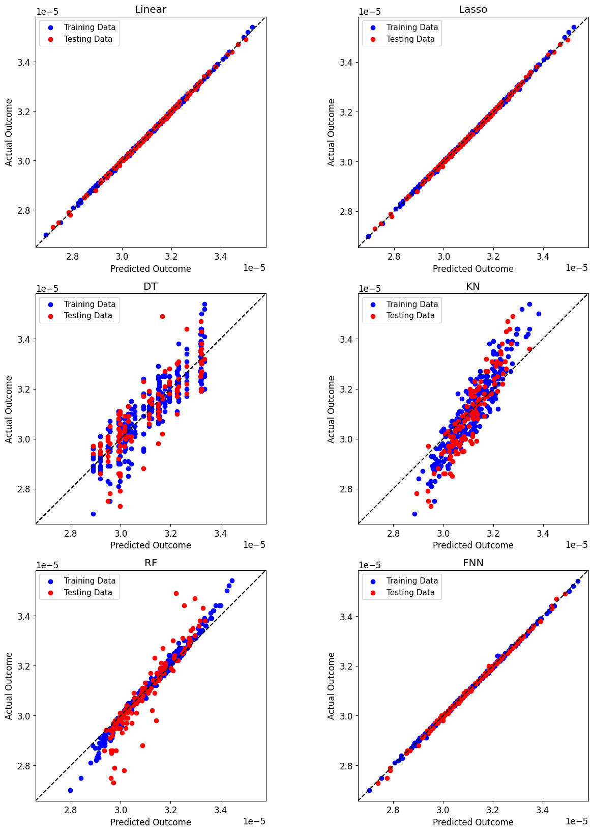
performance_plot(postprocessor.diagonal_validation_plot, "fis_gas_produced")
plt.show()

../_images/benchmarks_fuel_performance_35_0.png

[19]:

performance_plot(postprocessor.diagonal_validation_plot, "max_fuel_centerline_temp")
plt.show()

../_images/benchmarks_fuel_performance_36_0.png

[20]:

performance_plot(postprocessor.diagonal_validation_plot, "max_fuel_surface_temp")
plt.show()

../_images/benchmarks_fuel_performance_37_0.png

[21]:

performance_plot(postprocessor.diagonal_validation_plot, "radial_clad_dia")
plt.show()

../_images/benchmarks_fuel_performance_38_0.png

With these plots, we can see the narrow spread of Linear, Lasso, and FNN to \(y = x\), the best possible performance of a model. Additionally, KN appears to be overfitted to the training data set, and the predictions of FNN under 700 K approximate the max fuel surface temperature.

Similarly, the pyMAISE.PostProcessor.validation_plot function produces validation plots showing each output’s absolute relative error.

[22]:

models = np.array([["Linear", "Lasso"], ["DT", "KN"], ["RF", "FNN"]])

fig, axarr = plt.subplots(models.shape[0], models.shape[1], figsize=(17,20))

for i in range(models.shape[0]):
    for j in range(models.shape[1]):
        plt.sca(axarr[i, j])
        axarr[i, j] = postprocessor.validation_plot(model_type=models[i, j])
        axarr[i, j].set_title(models[i, j])
        axarr[i, j].get_legend().remove()

fig.legend(
    ["fis_gas_produced", "max_fuel_centerline_temp", "max_fuel_surface_temp", "radial_clad_surface_temp"],
    loc="upper center",
    ncol=4
)
plt.show()

../_images/benchmarks_fuel_performance_40_0.png

The performance gap between the linear model and the others is evident in the magnitude of the relative error.

Finally, the most performant FNN learning curve is shown by pyMAISE.PostProcessor.nn_learning_plot.

[23]:

postprocessor.nn_learning_plot()
plt.show()

../_images/benchmarks_fuel_performance_42_0.png

The validation curve is below the training curve; therefore, the best performing FNN is not overfit.

Fuel Performance

pyMAISE Initialization

Model Initialization

Hyperparameter Tuning

Model Postprocessing